Bitcoin’s Positive Skew

Positive skew in Residuals as well, for easier Trading: Lindy and Future Supply Models

This is not investment advice. Bitcoin is highly volatile. Past performance of back-tested models is no assurance of future performance. Only invest what you can afford to lose. You must decide how much of your investment capital you are willing to risk with Bitcoin. No warranties are expressed or implied. 

Look for Positive Skew: Taleb

In his Bleed or Blowup article for the Journal of Behavioral Finance, Nicholas Nassim Taleb notes that many investors seem to prefer repeated small positive payouts but thereby assume the risk of large negative drawdowns or blowups. One should seek positive convexity, positive skew instead, to maximize long-term returns. Fortunately we have Bitcoin, which exhibits strong positive skew.

For a summary of 20 reasons why Bitcoin is AntiFragile or positively skewed as a system and as a digital currency see: https://link.medium.com/OFT3aYbkM8

Jensen’s Inequality Shows Convexity

Positive convexity essentially means there is more upside than downside in an investment, and that its response to volatility is favorable. One might expect that Bitcoin itself has positive convexity, since if you buy it straight, not on margin, then the downside is limited to the cost, but the upside might be much more than the initial price, given it is new technology with a strong long-term trend, and provided you have sufficient patience (HODLing).

One can show that several popular Bitcoin price or market cap models demonstrate historical positive convexity using Jensen’s inequality.

The Jensen inequality takes the form:

E[F(x)] > F[E(x)] .

This means the expected value E of the model F built on input parameter x is greater than the model’s output for the expected or average value of the input parameter, E(x).

In the previous two articles of this series (https://stephenperrenod.substack.com/p/bitcoins-lindy-model and https://stephenperrenod.substack.com/p/bitcoins-future-supply-model) we presented the Lindy model as a power law in Block years elapsed (x = Block years of 52,500 blocks each) and a Future Supply model with an exponential relationship to the remaining fraction of Bitcoin yet to be mined.

The popular Stock-to-Flow model uses the stock-to-flow variable as the principal input parameter. All three of these are two-parameter models with a slope parameter and an intercept / normalization parameter.

All three models satisfy the Jensen inequality. One can calculate a Jensen inequality ratio given by the left hand side divided by the right hand side of the inequality relationship.

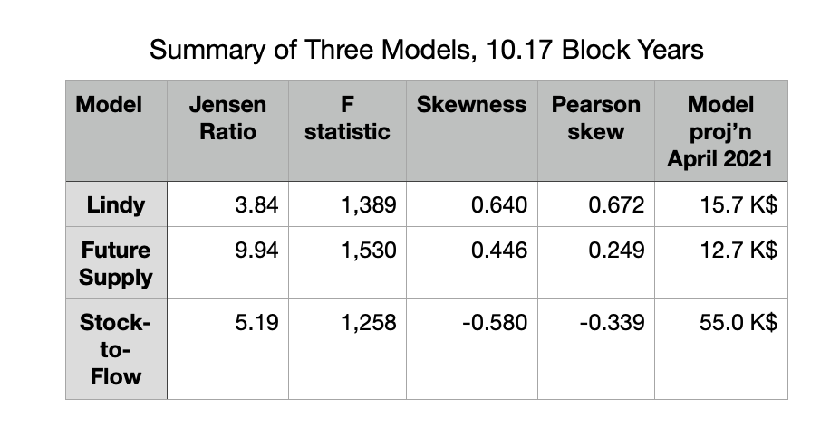
I have evaluated the Jensen inequality for each of the models using the respective best-fit slope parameters found over the period from 2 to 12 BlockYears elapsed. The Lindy model, Future Supply model, and Stock-to-Flow model have Jensen ratios of 3.84, 9.94, and 5.19 respectively.

The model regressions themselves have 123 Block monthly data points each, extending over the 10.17 Block years ending in July, 2020.

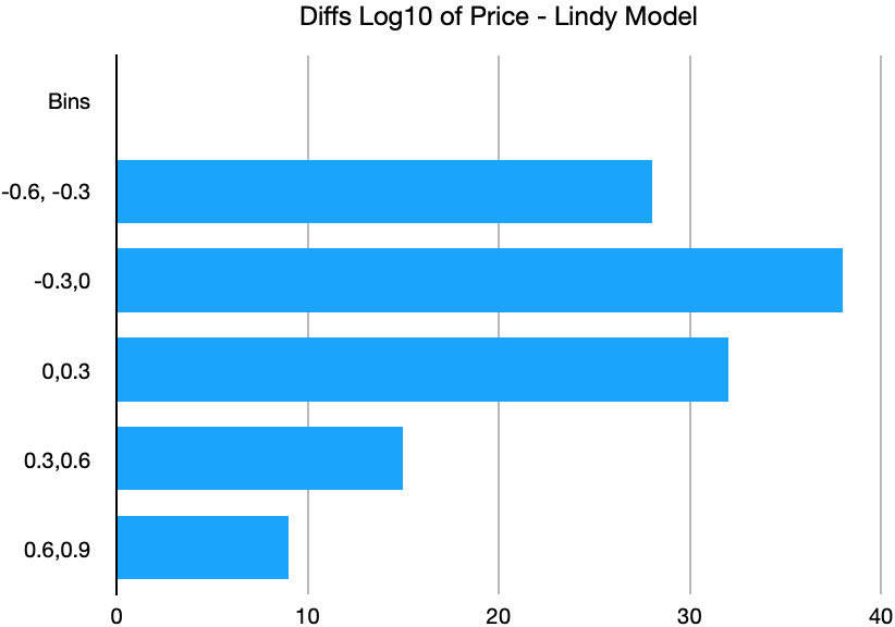
The Lindy model fits a power law relationship P ~ (Byr)^k with a best fit index k = 5.283 for the interval. The log10 residuals are shown in Figure 1; each bin represents a range in price of about a factor of two (0.3 dex or 10^[0.3]). Because of its dynamic price movement, its high volatility, it is best to think about Bitcoin price variation in logarithmic terms. Standard deviations for these models are above a factor of two in price.

As an example of the Jensen inequality calculation, we take the Lindy model with a power-law relationship between price and number of Block years elapsed, with best-fit index = 5.283. Thus, taking annual data points, the mean of the temporal interval is 7 Block years, and if that is raised to the 5.283 power we have 29,151. However the mean of the series 2^5.283 + 3^5.283 + …. +12^5.283 is 111,808. The Jensen ratio is thus much above one, at 111,808/29,151 = 3.84 and the model has high positive convexity.

Figure 1. Log10 Residuals for Lindy Model 

Residuals Positively Skewed for Lindy and Future Supply Models

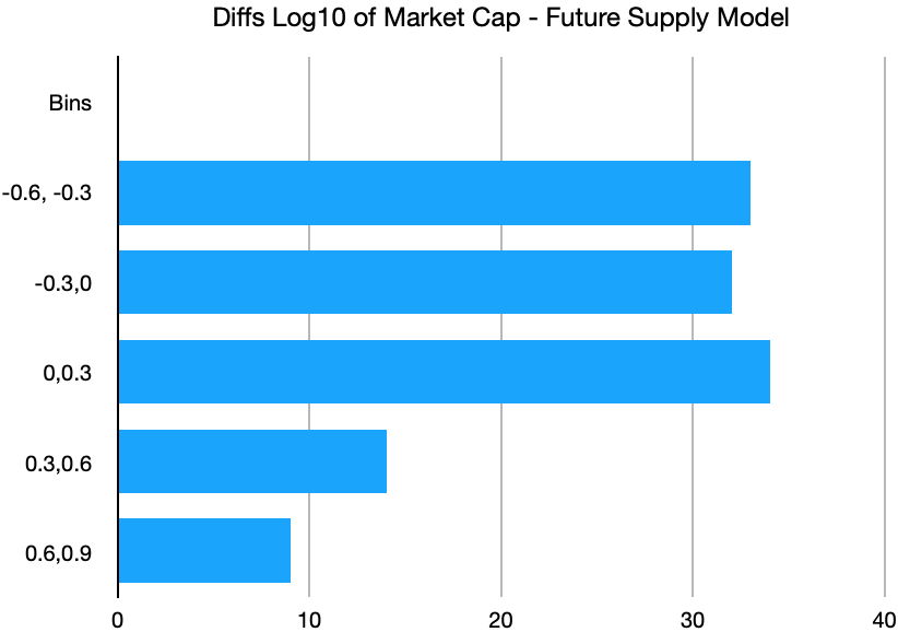
The Future Supply Model fits a relationship log 10 (MC) = b + a*f  where MC is the market cap, a is a slope parameter, b is log10 of the ultimate market cap B (around $1.4 trillion) and f is the fraction of Bitcoin’s 21 million supply not yet mined. In other words, the Market cap is an exponential in f, but with a negative slope. (It can also be cast as MC = B*10^(a*f) ; a takes a negative value). The log 10 residuals for the FSM are shown in Figure 2.

Figure 2. Log10 Residuals for Future Supply Model 

The residual histograms for these two models are somewhat similar and in both cases exhibit a positive skew with data points beyond 0.6 dex only on the right tails (thus, a factor of 4 or greater above the best fit value of price or market cap).

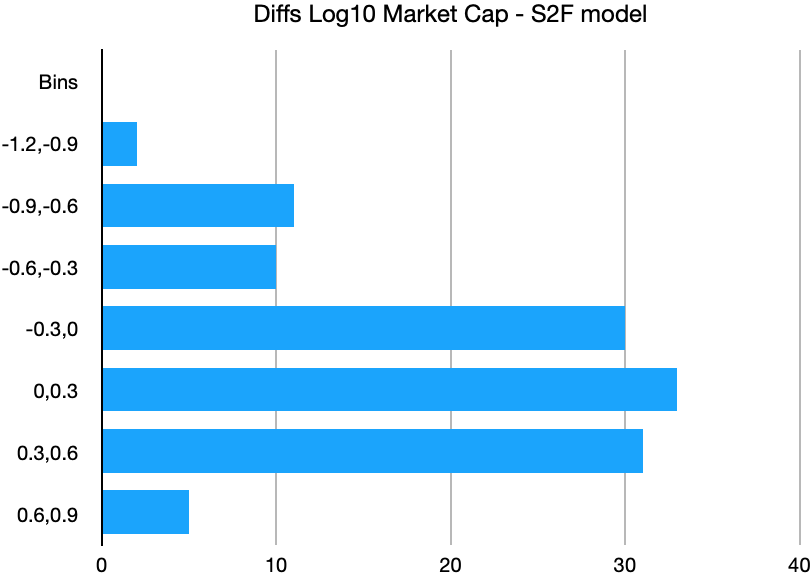
In Figure 3 we show the log10 residuals for a Stock-to-Flow power law model fit to market cap. (Stock to flow is calculated as the one Block year forward looking value at each data point). Here we see the residuals have a negative fat tail, with two additional bins. There is one data bin extending to over 0.9 dex away from the best fit, and the additional 0.6 to 0.9 dex bin is more heavily populated in the left tail than in the right.

Figure 3. Log10 Residuals for Stock-to-Flow Model

The Future Supply model has the highest Jensen ratio of the three models, It also has the highest F-statistic. The Lindy model has the greatest positive skew for its residuals. These values are all summarized in Table 1.

Because of the high volatility, Bitcoin is tricky to trade, but the volatility is where the opportunity lies. Almost any long term model shows a strong positive trend. One way to make trading easier is to adopt a model with positively skewed residuals.

One can calculate the positive skews for the Lindy Model and Future Supply Model residuals using both Skewness and Pearson Skew methods. The results are shown in Table 1.

These methods show the Lindy Model has the largest positive skew for its residuals, and also show the clearly negative skew of the Stock-to-Flow residuals.

For each of the three models, the long-term returns are positively skewed, but two have positive skew in their residuals, one has negative skew.

I assert that it is easier to trade a model that exhibits positively skewed residuals as well. The observed price spends less time below the model’s fair value in this case. I will present a specific trading strategy with six year back tested results in the next article of this series. Both the Lindy model and the Future Supply Model backtests show one can improve over a buy and hold strategy, by buying when the model residual is substantially negative and taking profits when the residual is significantly positive.

Table 1: Jensen ratios and Skewness parameters for three models