Bitcoin's Future Supply Model

A convergent integral supply driven model for Bitcoin market cap

“The portion of the integral calculus, which properly belongs to any portion of the differential calculus, increases its power a hundred-fold” — Augustus De Morgan 

This is the second article in a four article series. In the previous article I discussed a long-term Lindy model for Bitcoin’s price. In this article I present an overview of my Future Supply Model that is based on remaining Bitcoin reserves.

Both models exhibit positive convexity or skew to Bitcoin’s price volatility. This means they are antifragile, as is Bitcoin generally.

The Future Supply Model is a linear correlation of the log of market capitalization with the remaining Bitcoin supply yet to be produced (not yet mined) at any epoch. The mathematical form of the model is inherently convergent, whereas the popular Stock-to-Flow model is a power law of an exponential and thus is inherently divergent. Stock-to-flow is a differential of the supply.

More precisely, the Future Supply Model (FSM) is a two-parameter, convergent, residual supply-driven Bitcoin long-term forecasting model. It was created as an alternative to PlanB’s popular but mathematically divergent two-parameter scarcity-driven Stock-to-Flow (S2F) model. Over a 50 year time span, the models differ by a factor of a trillion in their Bitcoin fair value price estimate. 

Using the best fit parameters, the FSM converges toward an asymptotic value of market cap equal to $1.44 trillion (in 2020 dollars) and an asymptotic price of $68,300. However these values have high uncertainty due to the limited price history and high volatility of Bitcoin.

One should be able to easily distinguish whether the Future Supply model or the Stock-to-Flow model is more accurate by the mid-2020s.

This is not investment advice. Bitcoin is highly volatile. Past performance of back-tested models is no assurance of future performance. Only invest what you can afford to lose. You must decide how much of your investment capital you are willing to risk with Bitcoin. No warranties are expressed or implied. 

Motivation of FSM

FSM was motivated by the desire to have a convergent model that was also based on the increasing scarcity of new Bitcoin production. 

One possible analogy is to look at the valuation of a gold mine.

If you had a gold mine, how would you value it? You would not base your valuation for a gold mine using only a single year’s production. A stock-to-flow model, or differential model, does just that, it only looks at one year’s production relative to all prior production.

Rather, you would look at the reserves in place, and then estimate the cost of extraction, transportation, and refining. You would do this on a discounted cash flow analysis of this year’s production, and next year’s, and the year after that. You would go out into the future many years until the point at which you thought the remaining quality and quantity of reserves would make the mine uneconomic for further production based on your gold price forecasts, production cost inflation, interest rate forecast, and the like. And then you would add up all the discounted cash flows to arrive at a net present value of the gold mine.

This is not a perfect analogy, but since the value of Bitcoin is somehow related to all the expenses and profits of the Bitcoin mining industry, you get the general idea, hopefully.

The FSM looks at all future production relative to the production over the entire mining lifetime. In the case of Bitcoin, the mining production is everything from inception in 2009 until approximately the year 2140, or whenever the final total of 21 million Bitcoins is reached.

FSM Definition and Model Fit

The regression was performed over the ten Block Year interval, starting from 2 elapsed Block years (January, 2011) to 12 elapsed Block years, ending with the third Halving on May 11, 2020. It is simpler to create the model in Block calendar terms, and more natural as well, since difficulty adjustments and Halvings happen precisely on prescribed block intervals. Each Block Year contains 52,500 blocks and typically has a duration a few percent shorter than a regular calendar year.

For FSM, I looked at both power law and exponential relationships between market cap and future supply. The power law, or log (market cap) vs. log (future supply) model is divergent, since the latter term goes to negative infinity as the remaining supply goes to zero. While such a model has a reasonable R^2 for historical data, it predicts a market cap of $299 trillion when remaining supply drops to one million, less than six Block Years from now. This is equal to all global wealth, and is thus untenable. Any power law of index > 0.1 rises faster than global wealth can rise in real terms.

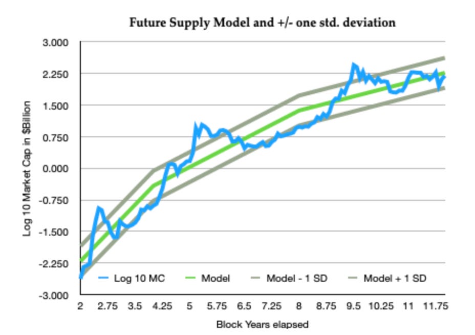
Figure 1 below shows the model fit to monthly data over a 10 Block Year period. 

Figure 1: Log10 of Future Supply Model market cap best fit curve (green) vs. observed Block monthly values of market cap (blue). Note the two breaks in slope of the model at the first and second halvings (years 4, 8). The market cap model is a monotonic function with slope discontinuities at Halvings. On this scale, zero on the ordinate corresponds to a $1 billion market cap, and three corresponds to a $1 trillion market cap. Also shown are the plus/minus one standard deviation curves. For the FSM, market cap heads toward an asymptote in constant 2020 dollar terms of around $1.4 trillion.

With the FSM, using an exponential relationship, the Bitcoin market capitalization (value of all currently existing bitcoins) is modeled as log 10 (MC) = b + a*f, where f is the remaining fraction of 21 million bitcoins yet to be mined, a is the slope (negative), and b is the log of the asymptotic market cap, reached when f = 0 in the next century. The fraction f is determined in a straightforward manner from the number of Block Years and Block Months elapsed (directly related to block height) and the Bitcoin Halving scheduled at each 210,000 blocks.

When market cap is measured in billions of dollars, the best fit parameters are a = -7.15 and b = 3.16, corresponding to an ultimate market cap equal to $1435 billion (2020 dollars). The price of one bitcoin is simply related to the market cap by P = MC/[(1-f)*21 million].

The Future Supply Model exhibits R^2 = 0.925 with 121 historical data points, one per Block Month. Block Months are each of duration 4375 blocks (1/12 of a Block Year). The residuals are well-behaved but clearly skewed positively. The standard deviation of the residuals is 0.355 in base 10 logarithm terms, reflecting Bitcoin’s high volatility. The R^2, Bayesian information criteria, and F-statistic all score well, and each scores better than the S2F model on the same data (with .925 vs. .918, -234 vs. -220, and 1466 vs. 1291, respectively).

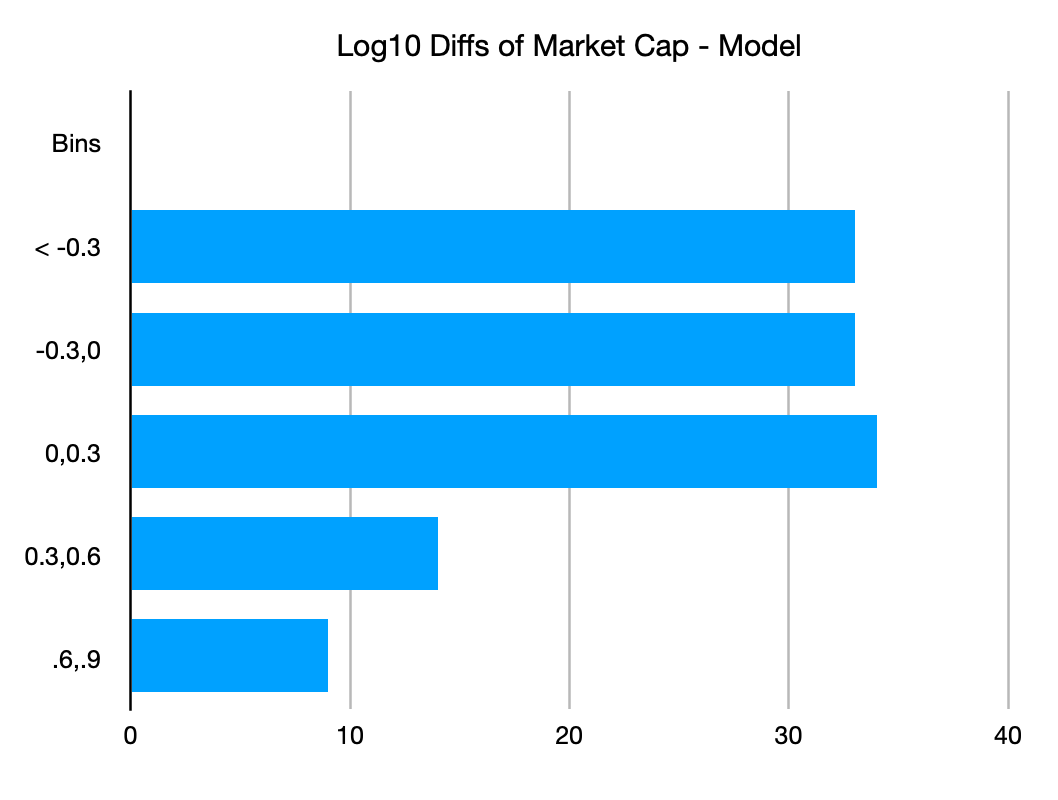
Figure 2 presents a histogram of model residuals, spaced at 0.3 dex (10^[0.3], or about a factor of 2 increase or decrease for each bin boundary). Note the asymmetry with a positive fat tail extending above 0.6 dex (factor of 4 difference and higher) but no corresponding tail on the negative side. There are only two negative bins, but three positive ones.

Figure 2: Residuals for the Future Supply model, binned at intervals of 0.3 dex (factors of two, approximately)

The clear positive fat tail suggests we have a model which could be favorable to trade as a long position. For example, we can accumulate in the first bin and take profits in the top two bins. In the next article of this series I will discuss the benefit of Bitcoin’s positive skew found with either the Lindy model or Future Supply Model.