Bitcoin's Lindy Model

Persistence drives Value

This is the first in a four article series in which I present two long-term models for Bitcoin value and backtest each with a particular trading methodology. Both models exhibit positive convexity or skew to Bitcoin’s price volatility. This means they are antifragile, as is Bitcoin.

In this article I provide an overview of a Lindy model of Bitcoin price vs. the block height or number of blocks in the time chain (blockchain). It is a price-time model in the Block calendar system. That system is close to the Gregorian calendar system but designed around the actual block count.

In the second article I will provide an overview of my own Future Supply Model (FSM). This model is a scarcity-driven alternative to the stock-to-flow model. Whereas S2F looks at the annual production only (inflation rate), the FSM is based on all remaining reserves of unmined Bitcoin. Unlike S2F, it converges to an ultimate value (in constant dollar terms).

The third article will show that for fits to both the Lindy model and the FSM, the residuals are positively skewed (convex). Convexity means the expected outcomes have a positive bias; the models are favorable to trade, with potential reward exceeding risk. We also show that a stock-to-flow model has residuals that are negatively skewed. That does not mean the model is not useful, but it is more challenging to trade.

The fourth article is a simple trading system and backtest over a six year period. For either the Lindy or Future Supply models the backtest results show far better results than a periodic purchase and HODL model.

This is not investment advice. Bitcoin is highly volatile. Past performance of back-tested models is no assurance of future performance. Only invest what you can afford to lose. You must decide how much of your investment capital you are willing to risk with Bitcoin. No warranties are expressed or implied. 

Lindy Model

Nic Carter has noted the applicability of the Lindy effect to Bitcoin. “Life expectancy is proportional to age.” This does not apply for adult humans, but it can apply for technology.

The Lindy effect is named after a deli in New York and was originally used in the context of comedians’ visibility and access to paid work. Nassim Nicholas Taleb, in Antifragile and other writings, has discussed it in the context of technology and memes.

The basic concept is that the longer a technology has been in existence and applied, the longer is its expected future viability. The wheel has been around a few thousand years (although we only started putting them under suitcases in the late 20th century). Electricity has been in houses a hundred years or so. These  technologies have staying power, persistence.

Bitcoin as a monetary asset is young in comparison to the monetary technologies of fiat dollars, double entry accounting, and gold. But every year that it persists and grows in value, its future becomes even brighter.

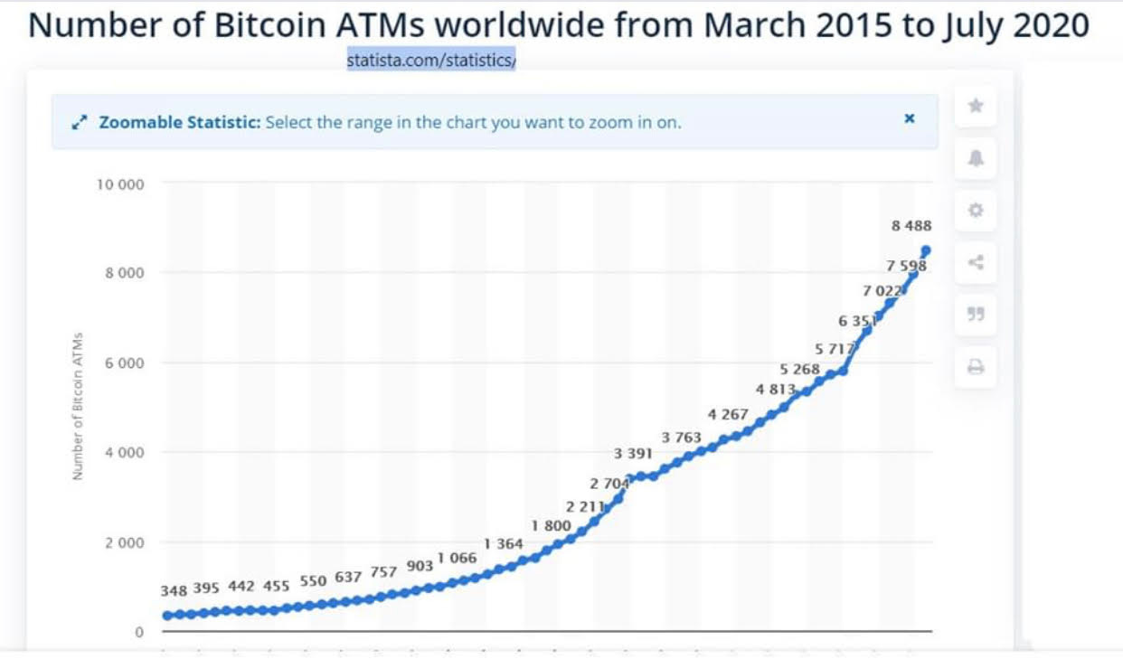
Figure 1: Number of Bitcoin ATMs grew over 20 times in 5 years, and roughly as the 6th power of the elapsed number of Block years (power law index 5.93, R^2 = .986).

The network effect grows as more and more people are introduced to Bitcoin, as more exchanges come into being, as use cases grow, as second layer solutions are introduced, as hash rate of miners increases, and as the value generally rises.

This Lindy model for Bitcoin’s price is very simple and easy to calculate. It takes the form of a power law between price and the number of blocks laid down. The latter can be more easily express in BlockYears. It is more natural and intrinsic to Bitcoin to fit a model based on block count, since mining difficulty adjustments and block subsidy Halvings are also based on block count.

In the Bitcoin calendar system, one Block Year is 52,500 blocks and has been running a little less than one calendar year. We are now in Anno Satoshi 13, since a little more than 12 Block Years have elapsed since the first block in January, 2009.

I discussed the Lindy model in a previous post: https://stephenperrenod.substack.com/p/bitcoins-pre-determined-disinflationary where I noted that the price can be modeled using a power-law relationship,

P ~ (Byr)^k ,

where Byr is the number of elapsed Block years, and k is the power-law index.

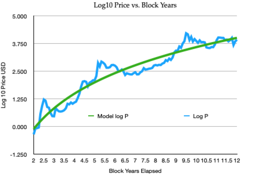
Figure 2 shows the model historical fit, here updated with Block monthly prices starting from BYr = 2, through the third Halving on May 11, 2020 with BYr = 12 elapsed Block years. 

Figure 2: Observed Blockmonthly prices and a fit with a Lindy power-law model of index k = 5.289

The best fit line of log10 (P) = m + k* log10 (Byr) has a steep index, k = 5.289, reflecting the rapid overall price rise. The model has a logarithmic (base 10) standard deviation of 0.334, an R^2 of 0.918 and has a Bayesian information criterion of -249 and an F-statistic of 1331.

It projects fair value prices of $23,304 by early 2022 and $65,078 by 2025.

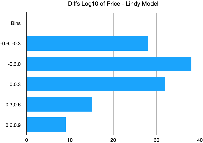
Figure 3: Residuals for the Lindy model, binned at intervals of 0.3 dex (factors of two, approximately)

Figure 3 is a histogram of model residuals, spaced at 0.3 dex (10^[0.3], or about a factor of 2 increase or decrease for each bin boundary). Note the asymmetry with a positive fat tail extending above 0.6 dex (factor of 4 and higher) but no corresponding tail on the negative side.

The Lindy model is phenomenological; it does not have a precise underlying motivation. It reflects the growth in the ecosystem and longevity of Bitcoin, supported by its antifragile nature. It implicitly reflects the increased security of a lengthening blockchain with rapidly increasing hash power behind it. And it reflects the increasing scarcity as the amount of new Bitcoin created is decreased, cut in half, at each Halving interval.

I will discuss this more in the third article of the series, how volatility helps Bitcoin. In the next article we briefly describe the Future Supply Model.