Two-Year Scenario for Bitcoin: Two Log-Periodic Modes
Flat 12-Month Outlook, Next LP Peak around 2030

Executive Summary
Bitcoin’s global median power law remains robust, β = 5.848 and descriptive R2 = 0.958 for a QR regression.
Two global log-periodic modes raise the overall descriptive R2 to 0.980.
Re-estimating modal amplitudes and phases over the latest five years explains approximately 87% of residual variance in that window.
The five- and eight-year scenarios suggest broadly flat behavior over the next year, followed by recovery during 2027–28; these are conditional scenarios, not precise price targets.
Background
Bitcoin resembles an astrophysical system in one important respect: we can observe it with increasingly sophisticated instruments, but we cannot run controlled experiments on its development. Short-term prices can be influenced by exchanges, derivatives, and market structure, but the longer-term phenomenon is the evolution of a self-organizing monetary network. Consensus, security, adoption, liquidity, and perceived value develop jointly through reinforcing feedback loops that have no close analogue among conventional currencies, commodities, or equities. Major currencies and commodities have been falling in power law terms relative to Bitcoin over its lifetime.

It has been well established that Bitcoin follows a long-term power law with a very robust R2 of 0.96 (A Mechanistic Derivation of the Bitcoin Price Power Law: Network Adoption Dynamics and Generalised Metcalfe Scaling, Giovanni Santostasi and Stephen Perrenod DOI: 10.5281/zenodo.19387099).
Since a year ago as I saw that no significant bubble above the power law trend was appearing during 2025, I have been developing log periodic models of the price residuals that remain after subtracting out the power law. Structural log periodicity in Bitcoin is well-supported by peak and trough spacing, by FFT, Lomb-Scargle, and wavelet spectral analysis, and by fits to price history.
We have suggested that the power law and the log periodicity are both expressions of the underlying network. The relationship C = 2π β/ω = β ln λ ~ 4 describes a candidate coupling invariant — a hidden variable between the power law with exponent β and a fundamental angular frequency of log periodicity ω ~ 9, (spacing λ ~ 2 in log age, related via ln λ = 2π /ω). The hypothesis is that β and ω are respectively the real and imaginary components for complex scaling, s = β + i* ω, such that taking the real part of ts = tβ * e{i* ω ln t} produces a power law modulated periodically in log time.
In Bitcoin’s Not so Hidden Structure https://stephenperrenod.substack.com/p/bitcoins-not-so-hidden-structure I showed that adding one or two log periodic modes improved out-of-sample forecasting over the range 6 to 24 months forward, relative to the power law, which itself performs better than all other models for horizons of 12 months and longer.
In Forecasting Bitcoin beyond the Power Law https://stephenperrenod.substack.com/p/forecasting-bitcoin-beyond-the-power I showed that medium-term localization substantially improves the model’s explanatory power. Holding the globally identified log-periodic frequencies fixed while re-estimating their amplitudes and phases over a trailing five-year window increased the proportion of recent power-law residual variance explained by two modes to as much as 82%. This suggests a useful separation: the frequencies may reflect persistent global properties of Bitcoin’s scaling structure, while their amplitudes and phases evolve (drift) with the network’s local dynamical state.
The declining percentage size of successive bubbles suggests that constant-amplitude log-periodic coefficients are inadequate over the full history. This motivates allowing amplitudes and fitted phases to vary over intermediate-term windows. Phase drift is also expected in dynamical systems of this nature.
Procedure
The procedure followed here was to fit the fundamental parameters β and ω globally, but to use intermediate-term local fits for the amplitudes and phases of two log periodic modes. The fundamental and second LP mode frequencies were determined from a Lomb-Scargle fit (similar to an FFT analysis for dominant frequencies, but more suited for log spacing analysis). In the earlier work we had good results with a 5-year window, here we looked at 3, 4, 5, 6, and 8-year windows and found that the two shorter ones were insufficiently short to capture intermediate term parameters.
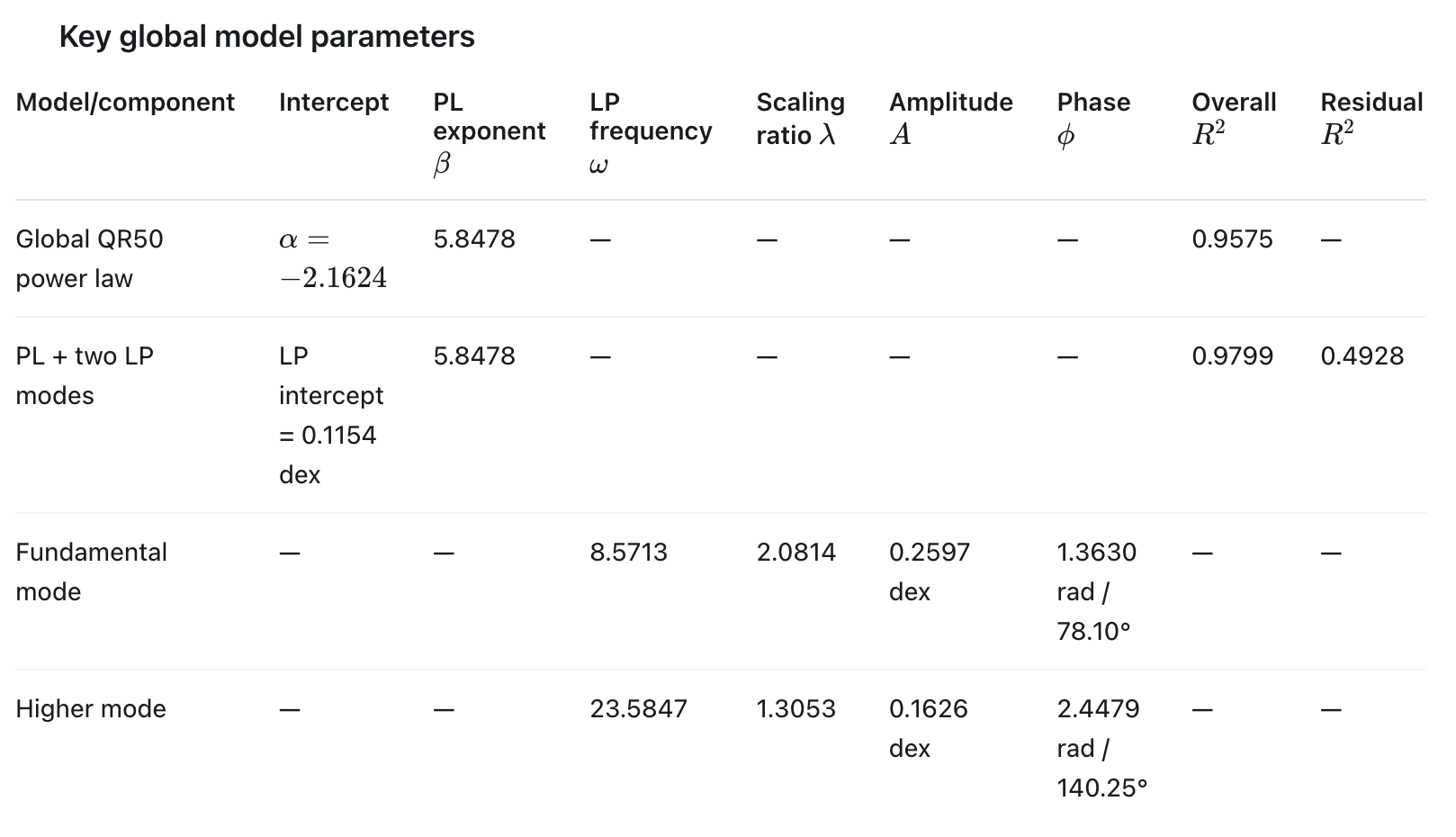
Table 1 reports the globally estimated structural parameters. The global power law explains 95.8% of the variance in log price, while adding two globally calibrated log-periodic modes raises the overall descriptive R2 to 0.980 and explains 49.3% of the remaining residual variance. When the two frequencies are held fixed but their amplitudes, phases and intercept are re-estimated over the latest five-year window, the two-mode model explains approximately 87% of the residual variance within that interval. This large local improvement motivates using five-year coefficients for the conditional forecast scenarios below.
Robustness
As a leakage-free robustness check, I repeated the exercise from earlier forecast origins using five- and eight-year local windows and six- and twelve-month horizons. Overall, the power-law baseline outperformed the localized two-mode forecasts, although the five-year model modestly improved one six-month prediction. These limited tests do not establish out-of-sample superiority and indicate that locally estimated amplitudes and phases can be unstable. The current projection should therefore be interpreted as a conditional endogenous scenario rather than a validated point forecast. These results do not negate the evidence for globally calibrated log periodicity; rather, they show that repeatedly localizing amplitudes and phases introduces additional estimation risk.
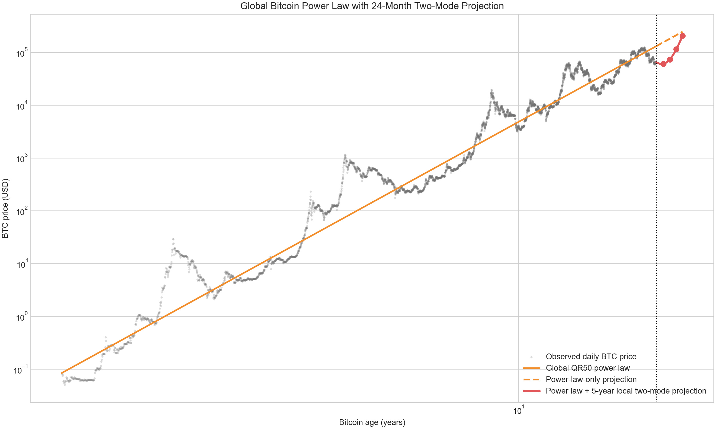
Power Law and Overall 2-year Projection
Figure 1 shows the median quantile-regression power law fit and also a two year projection with a 5-year training window for the two LP modes, on a log-log-scale. Note the three largest bubbles are approximately equally spaced in log time. The more recent bubble structure has influence from the higher mode, whose amplitude of 0.16 in log10 price is of the same order as the 0.26 amplitude fundamental. And for the most recent 5-year window the higher mode grew to an amplitude exceeding that of the fundamental (shown below). Growing power in non-fundamental modes is another typical aspect of this class of dynamic systems.