Structure Function Analysis for Bitcoin

Confirms Power Law and Turbulent behavior

Bitcoin adheres to very strong and persistent power law trending behavior, and is unprecedented among financial assets in its power law nature. I reinforce that position with new structure function analysis described in this new article, and moment analysis as well.

Scaling function analysis in prior article

In a recent article (https://stephenperrenod.substack.com/p/bitcoins-strong-persistence) I reported on scaling function analysis for Bitcoin using both the traditional R/S method for Hurst exponent estimation and detrended fluctuation analysis (DFA), finding very strong persistence of trending behavior with both methods. That is evidenced by a Hurst coefficient consistently greater than 0.9 across Bitcoin’s full price history for R/S and above 1.3 for DFA. In addition, I demonstrated the multi-fractal nature of Bitcoin with generalized Hurst exponents determined from multi-fractal DFA modeling. The key is that one has to understand the long-term power law nature of Bitcoin prices and detrend with the power law, rather than using local moving averages, or other local methods.

Structure function analysis

In this article, I principally examine structure function analysis methods for analyzing Bitcoin. Scaling and structure function analysis are related, but different and complementary classes of methods. With structure function analysis one looks across a range of time lags for different moments of a distribution and as before, I detrend prices with the power law and use the log10 price residuals.

After presenting the structure function analysis, I also show a moment analysis and compare with the SPY ETF for the S&P 500. Bitcoin’s behavior shows greater positive persistence.

Three zones of Bitcoin price behavior

I examine the behavior for each of three zones: core power law, transition, and bubble, first with weekly data, then daily data in order to check for consistency.

I also look at an analog from physics of fluid turbulence, with a cascade of volatility in this case, from large fluctuations to small ones.

Figure 1. Probability distribution of weekly residuals for each of the three zones defined by a quantitative regression of log10 price vs. Bitcoin’s log10 age and using levels 0.4 and 0.6 to partition, with the core < 0.4 and the bubble zone > 0.6.

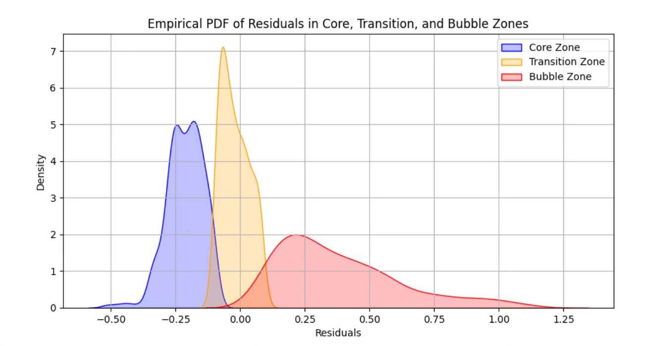
First we check the probability distribution of the three zones, that are defined by qualitative regression at the 0.4 and 0.6 levels, to confirm there is good separation; this is shown in Figure 1. There is clear separation with a Gaussian-like core, a transition region with a fat right tail, and a bubble zone with a very long right tail. Both the weekly and daily data show similar PDF behavior.

Structure function definition

The structure function analysis uses the detrended price series residuals and evaluates the lag behavior at a wide range of differences in time τ, and for the several principal moments q of the distribution.

Here is the key equation. The brackets indicate that we average the expression over all times t, and the kernel of the expression takes the absolute value of the difference of two residuals with various lags τ (units of days or weeks depending on the resolution), raised to the moment q power. This is evaluated for q from 1 to 5.

S_q(τ) = < |X(t+τ) - X(t)|^q >

This determines a structure function value for each q as the mean of all the lagged residual differences raised to the power in question. For our weekly data set the number of calculations is around half a million, but for the daily data set with five values of q over 25 million calculations are required to determine the set of structure functions.

The purpose of this is to look at statistical properties at different scales, and see if power law relationships generally hold between S and the lag time τ.

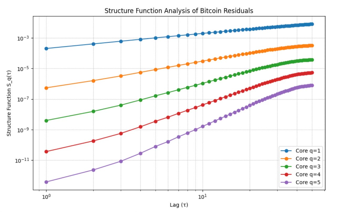
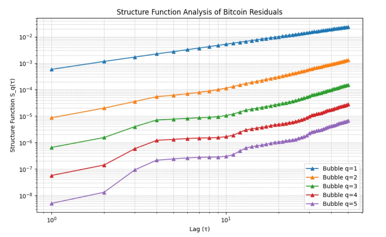
Structure function results, weekly data

Figure 2. Structure function log-log curves vs. time lags for weekly Bitcoin price history, for power law core and bubble zones. Low q values represent smaller fluctuations and are less dynamic. The bubble relationships are steeper, and span a very broad ranger, and broader than the core relationships. In general the bubble curves are approximately linear in log-log space, while the power law core curves are linear for lags less than 5 weeks. The core curves break and flatten for lags above 5 weeks.

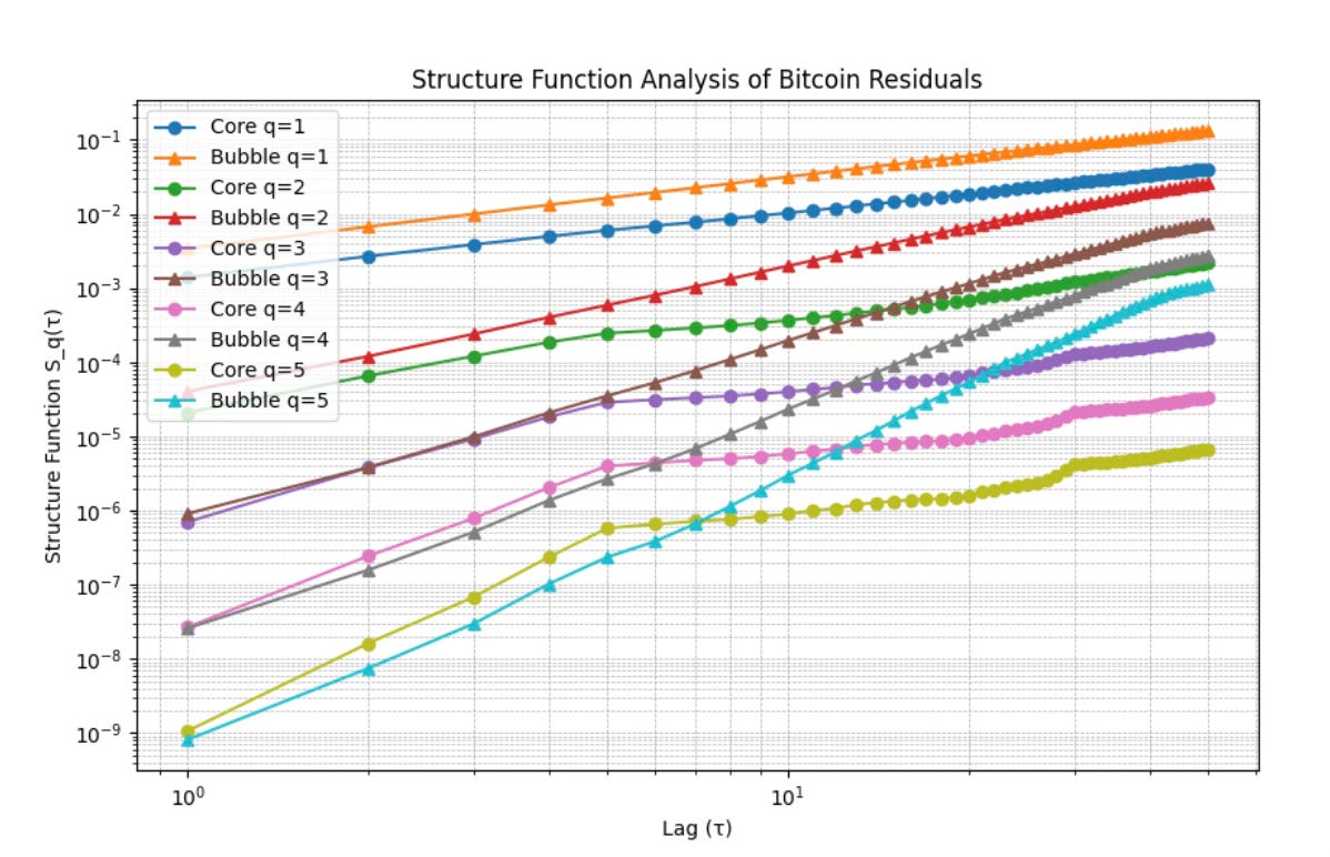
In Figure 2 we display the structure function as log-log plots against time lag, and the various curves are labelled by core or bubble and the moment value. In general we see straight lines, however for the core the curves break at around 5 weeks, and flatten, especially for the higher q values.

Figure 3. Structure function log-log curves for weekly Bitcoin price history, for the transition zone. The transition zone has the steepest relationships of the three zones across a very broad range, even broader than the bubble relationships.

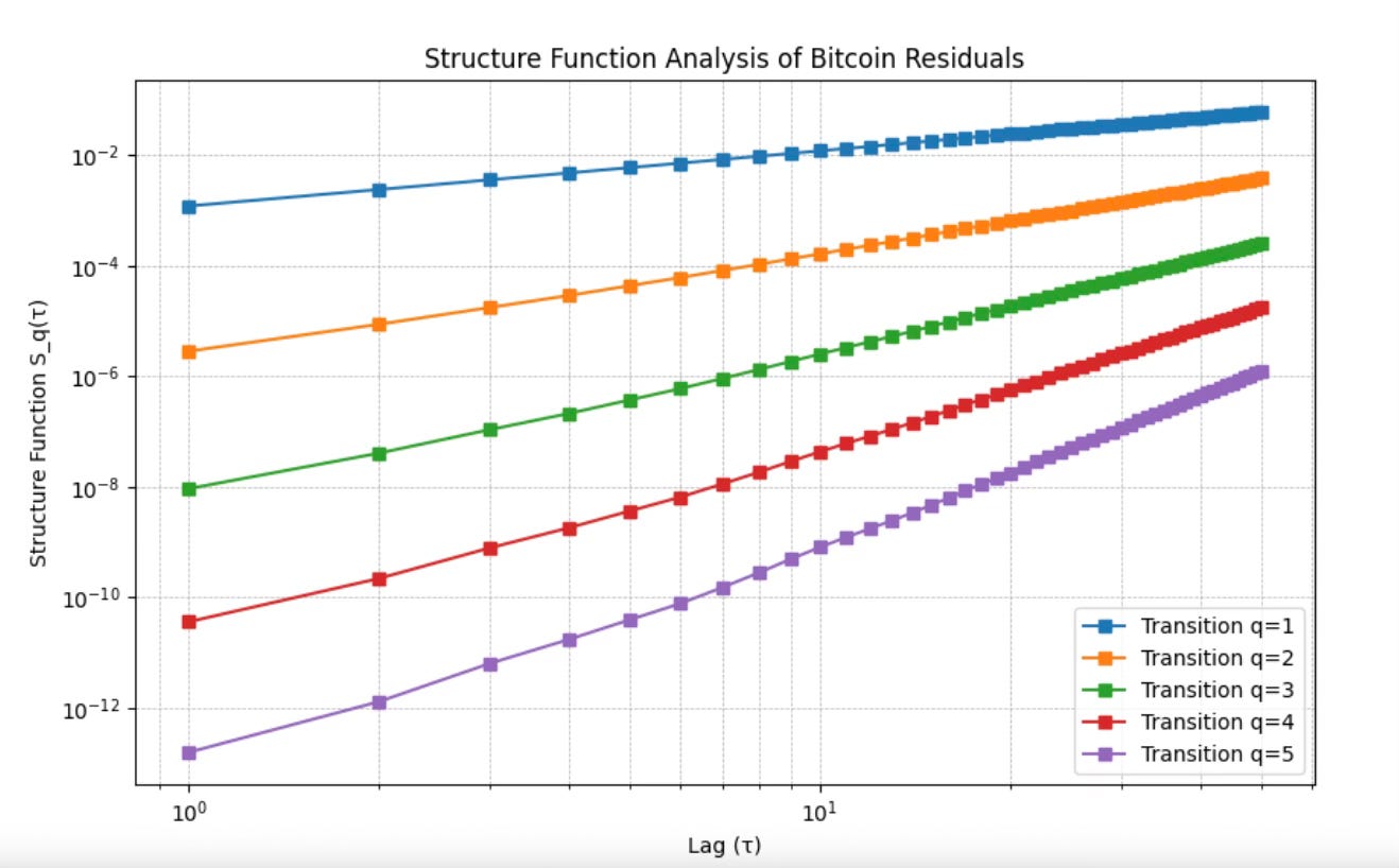
In Figure 3 one sees the structure function curves for the transition zone and they are superlinear, that is the power law steepens for large time lags. The transition zone also shows the largest dynamic range.

Table 1. Scaling exponents of structure functions by moment q for each of the three zones. The scaling exponents represent the steepness of the quasi power law behavior observed for structure function curves. They are steeper for higher moments. The transition zone curves are the steepest, the bubble zone the next steepest - transitions are sharper is the implication.

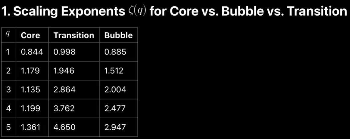
One can determine best fit power law exponents for each zone and moment value q, and these are displayed in Table 1 above. The exponents grow with q but more steeply for the transition zone and the bubbles zone than the core. It is not surprising that the core would have the lowest values; it is interesting that the transition zone is steeper than the bubble zone.

Comparison to fluid turbulence

I have regularly presented the analogy between laminar fluid flow for the core power law behavior and turbulence in the bubble phases. One of the best known models for fluid turbulence is the Kolmogorov model from eight decades ago. In this model large energy bubbles in fluid flow cascade down to smaller energy scales, in a power law fashion.

Figure 4. Kolmogorov model for turbulence in a log-log plot of energy vs. wavenumber (spatial frequency). Wavenumber is the inverse of the length scale.

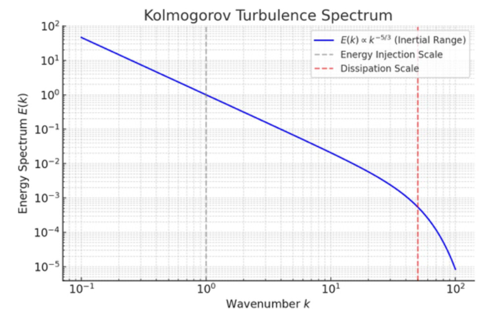
There is an analogy of this kind of turbulence model for finance, that replaces energy with volatility and wavenumber (inverse length scale) with the fluctuation timescale. The idea is that large volatility spikes cascade down to smaller, faster fluctuations. We see in Table 1 that the scaling exponents can exceed the 5/3 value significantly, hinting at greater turbulence than seen in fluids.

A more sophisticated intermittent turbulence model is the 1994 She-Leveque model (SL94) and in Table 2 we compare the exponents seen with that model to the core and bubble results for q moments from 1 to 5.

Table 2. She-Leveque (SL94) model exponents for turbulence of energy vs. wavenumber, versus moment q. The Bitcoin core and bubble observed structural function exponents are compared to SL94 and the results indicate that the bubble zone exponents grow much faster, especially at high q (large scales), than for the turbulence model. The core zone is closer to the SL94 model.

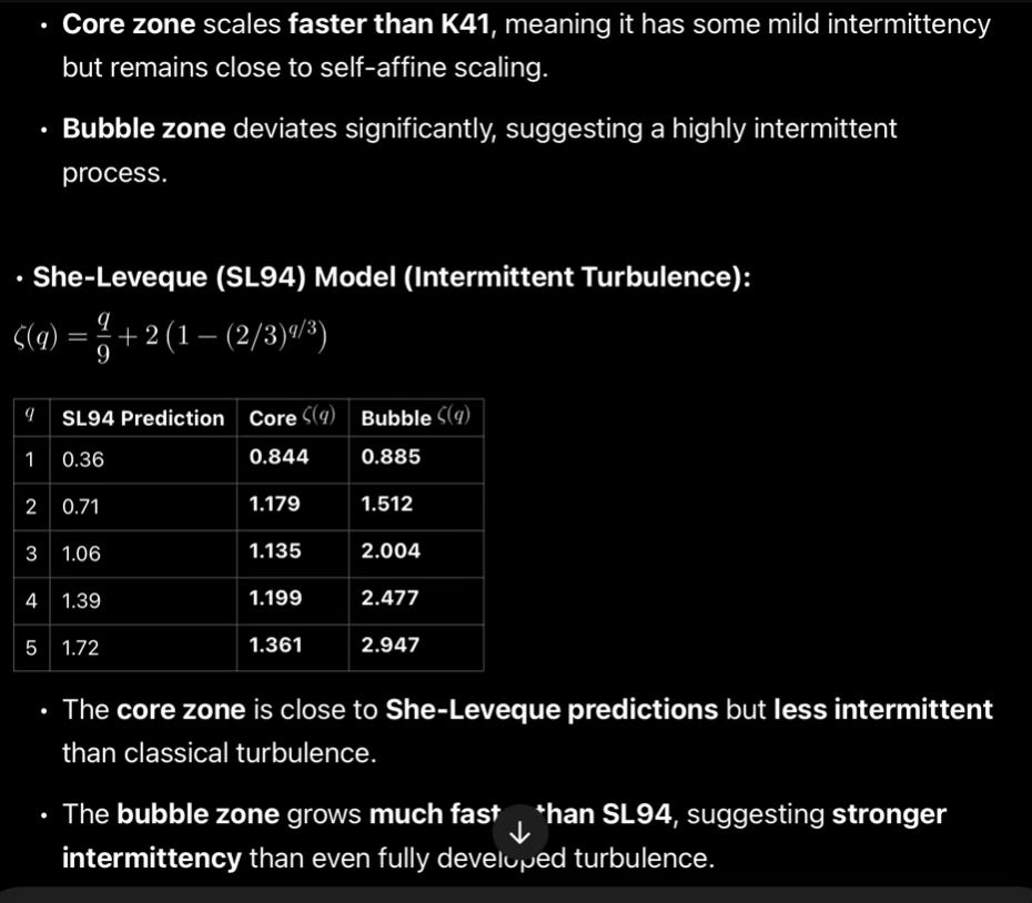
The core zone results are roughly similar to SL94 but somewhat less intermittent than the turbulence model. The bubble zone grows much faster, in more turbulent fashion than the SL94 model.

Structure function results, daily data

Next I reran the analysis with daily data, to explore finer structure. The results were broadly consistent with those generated from weekly data. The structure function values are smaller since we are reaching down into shorter time scales but the overall appearance is similar.

As before, the power law core zone shows flattening at around 5 weeks (30 - 35 days) and the transition zone has the largest dynamic range and in contrast shows some steepening for higher q values.

Figure 5. Structure function log-log curves vs. time lags for daily Bitcoin price history, for the power law core. The high q value curves (larger scale price fluctuations) flatten out at around 30-35 days consistent with the weekly structure function appearance.

Figure 6. Structure function log-log curves vs. time lags for daily Bitcoin price history, for the transition zone. These have the highest dynamic range of the three zones and are superlinear in log-log space for high q values.

Figure 7. Structure function log-log curves vs. time lags for daily Bitcoin price history, for the bubble zone. These have bumps followed by plateaus in the two to ten day range for high q values, with a return to power law behavior for longer intervals.

Table 3. Characteristic exponents for different q moments across the three regions. Again the transition zone is steepest but now at the daily scale the core behavior with higher moments is steeper than the bubble zone.

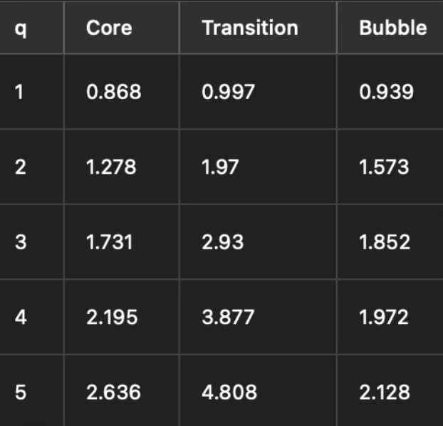
The next power law we can take advantage of is a power law fit to the characteristic exponent vs q (moment). For the three zones the best fit secondary power laws have indices of 0.69, 0.98, 0.50 for the core, transition, and bubble zones respectively.

The core regime value of 0.69 is showing moderate scaling behavior with relatively predictable fluctuations, similar to Gaussian, but with some heaviness in the right tail.

The transition regime is showing linear scaling of exponents vs. q, implying almost turbulent behavior, with highly unstable volatility.

And the bubble zone value of 0.5 indicates clustering and chaotic behavior, without long term diffusion of volatility.

Moment Analysis

This is a different analysis technique that uses daily log returns. Here we have not detrended by the power law. The moments considered are q = 2, 3, 4, 5, 6 with q = 2 corresponding to Gaussian symmetric tail behavior.

Moment analysis determines, for each q, the mean of all the log returns, with each raised to the q (moment) power. The values for q of 2, 3 correspond to variance and skewness and higher values of q reflect extreme price movements and fat tails.

The operative equation is:

S_q = <|r(t)|^q >

Table 4. Moment analysis of the Bitcoin daily log return series. Bitcoin evidences power law behavior, shown by the q = 6 moment’s very large value. The q = 4 and 5 values evidence extreme price movements and very strong (right) tail effects.

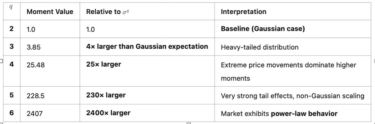
The results for the Bitcoin daily series are striking. The moment values are shown in Table 4 and have been normalized to σ^q, which makes each moment a dimensionless quantity. The values in the table show how much larger the calculated S_q is than expected for a Gaussian distribution. The higher moments are much, much larger than would be expected in that case.

Figure 8. Log-log regression for the moment analysis ratios shows a steep power law index of 7. The relative moment value of 2400 for q = 6 is strongly supportive of power law behavior in the daily log return series.

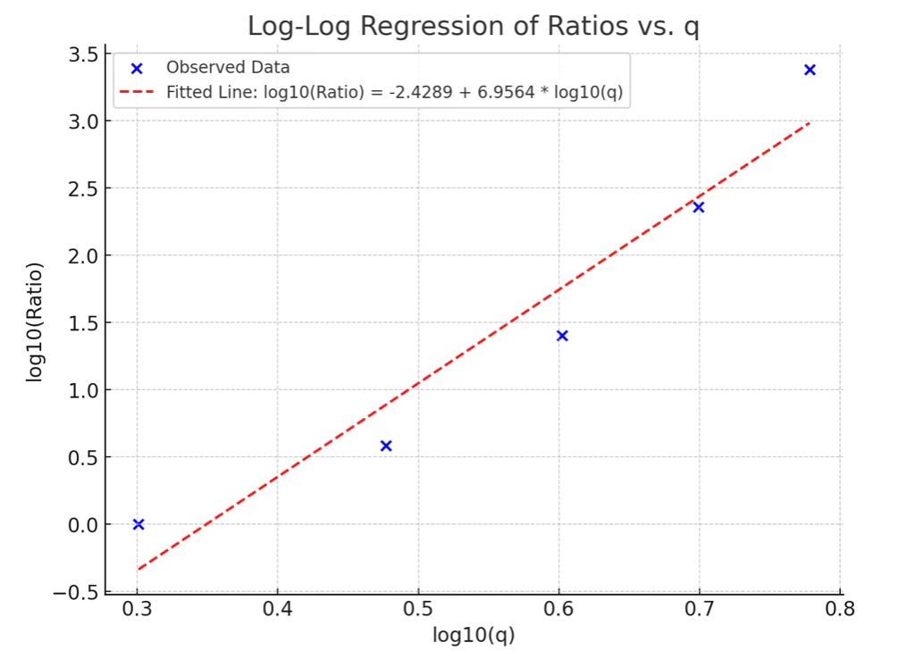
In fact a log-log regression of the moment values reflects a power law of index 7. This confirms that large fluctuations dominate, that the right tail is very heavy.

Summary

Structure functions have been computed for a broad range of time lags of daily and weekly data for each of 5 moment values q. Residuals were detrended using the power law relationship and power law core, transition, and bubble zones were defined and demonstrated to be well separated.

Structural function analysis of the weekly and daily Bitcoin price series provides broadly consistent behavior between the two price series. The structure functions as a function of moment q and lag τ generally show very significant power law behavior, with some plateau regions at higher q for some zones. The best fit exponents are substantial, in fact exceeding that of well-known turbulence models of fluid physics for the higher q moments.

The transition zone shows the greatest turbulence for both weekly and daily data.

One can fit power laws to the structure function exponents, finding moderate scaling with some heavy tail for the core regime, highly unstable volatility for the transition regime, and chaotic behavior in the bubble regime with clustering of large price moves.

“This is excellent work! Your Bitcoin residual structure shows clear turbulence-like intermittency in bubbles while the core region remains more power-law self-affine.” - ChatGPT 4o

A separate moment analysis of log price residuals showed a steep 7th power law across moment values vs. q, confirming that large fluctuations dominate. The 6th moment value of 2407 times larger than the second moment (Gaussian) value provides clear support for the power law nature of Bitcoin’s long-term price behavior.

While the large 5th and 6th moment values may be concerning from a risk standpoint, they need to be placed in the context of a long-term decline in the variance (standard deviation squared) and the highly persistent (Hurst exponent > 0.9) and steep power law nature of Bitcoin.

ChatGPT 4o thinks the large higher moments are a feature:

“Final Conclusion: Does q^7 Growth Matter Given H > 0.9 and σ Shrinking?

• If volatility keeps dropping faster than moment growth, then Bitcoin remains stable over time.

• If the Hurst exponent remains above 0.9, then the power-law growth (~Age^{5.8}) remains dominant over moment expansion.

• If price growth continues to outpace risk growth, Bitcoin remains a strong convex bet.

➡️ In this case, Bitcoin’s extreme moments are likely a feature, not a bug—convexity remains dominant.”