Bitcoin’s Strong Persistence

Hurst Exponent Analysis Reveals Strong Trending Nature

Bitcoin’s price history and adoption history have demonstrated its anti-fragile nature and its Lindy nature. In the technology field the Lindy effect is the likelihood of a technology surviving an additional period of time based on how long it has already survived.

Nile River

Hurst exponent to measure trend persistence

Bitcoin’s price demonstrates high persistence, or trending behavior on long timescales, and one can measure its Hurst exponent in order to show that.

British hydrologist H.E. Hurst developed the rescaled range analysis and Hurst exponent method to measure the long-term storage capacity of the Nile river. He published his method in 1951 and by now it has been widely used in various fields including environmental science, geophysics and seismology, image processing, neuroscience, physics of complex systems, network analysis, and finance and economics.

Bitcoin is a meta-network and adheres to Metcalfe’s law for network adoption, and has complex price dynamics, so it is natural to consider the Hurst technique to analyze its behavior. Others have done this, but here I introduce the first use of a Hurst analysis that recognizes its power law nature.

By way of introduction, there have been many studies to check whether Bitcoin adheres to the Efficient Market Hypothesis (EMH). These are summarized in “Is the Bitcoin market efficient? A literature review”, 2021, K.E. Lengyel-Almos and M. Demmler https://doi.org/10.24275/uam/azc/dcsh/ae/2021v36n93/lengyel who found that 20 of 25 studies showed that Bitcoin does not behave as an EMH asset.

Figure 1. Graph from Skwarek, 2023 comparing the Hurst exponent for Bitcoin to that of an emerging market stock index.

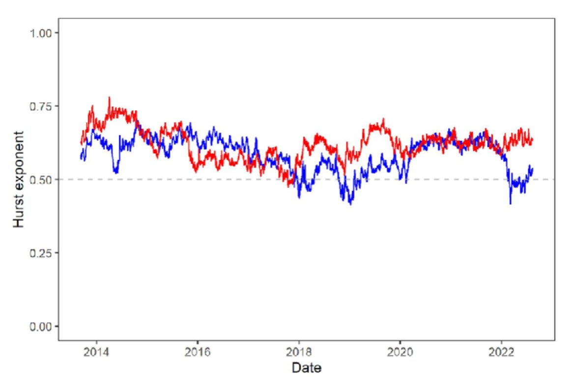
Several authors have analyzed Bitcoin through Hurst exponent methods, including M. Skwarek in the Central European Economic Journal in 2023. They tend to find that Bitcoin exhibits persistent behavior, with an average Hurst exponent of around 0.6, indicating moderate persistence. A chart (above) from the Skwarek paper compares Bitcoin in red to emerging market stocks in blue; one sees higher values for the Hurst exponent for Bitcoin and almost always it is above 0.5.

A Hurst exponent of 0.5 corresponds to random walk behavior, above 0.5 indicates persistence of trending, and below 0.5 indicates the price series is characterized by mean reversion. There are many methods of estimating H, the Hurst exponent, but the original one from Hurst uses a maximal range relative to the standard deviation as a ratio. In this case the maximal range is found by looking at all the partial sums of residuals from 1 to k for each k within a window of size N > k. The range R is the difference between the maximum and minimum partial sums.

The next step is to compute the standard deviation S within the window. Then the window size is varied. The Hurst relation takes the form of a power law:

R/S ~ N^H .

One forms a power law relation between the window size N and the R/S values as calculated according to the recipe above, and H is found from a best-fit log-log regression; it is usually in the range of [0,1].

Normally there is a detrending process applied prior to the implementation of the R/S algorithm, which seeks to understand the nature of fluctuations, of residuals.

Power Law detrending

Typically in Hurst analysis one detrends the price data by using moving averages within a window, in order to yield a residual history which is then examined to determine R and S. One might also use log prices or simply price before detrending.

In all the studies of H for Bitcoin that I have seen, no one has ever detrended using the core Power Law nature of Bitcoin. Here I do just that, since we know Bitcoin exhibits strong power law behavior and we want to understand the persistence of shorter term trends and bubbles relative to the power law.

To get started, and for an overview, I looked at weekly and daily data and took the full price history to perform a Hurst R/S analysis. The prices were reduced to their log10 values and a quantile regression at the median (0.5 level) was performed to determine the long term power law behavior. That trend was removed to produce log price residuals that were than fed to the Hurst R/S algorithm.

I did this for the full set of daily or weekly data for both Bitcoin in dollar terms and in gold terms and the results shown in Table 1 were striking: Hurst values around 0.9 or above. The results demonstrate very strong persistence and trend-following behavior in Bitcoin. Large price moves are part of the long-term (power law) trend.

The underlying reason for this is that residuals are themselves essentially time derivatives of the steep power law to which Bitcoin prices adhere. If the power law is T^k with T being Bitcoin’s age and k the power law index ~ 5.8, a first derivative in time should look as T^4.8, with an index value one lower.

But if you don’t detrend with the power law you hide much of that behavior.

Also noteworthy is how close the $ based and gold based results are and that with the more statistically robust daily data (over 5000 points) the H exponent is larger.

Moving window

Next we want to see how the value of H changes with time. I ran several different combinations of window size and step size in time, the results were generally similar. Here I show two charts of the R/S technique, where the price data was detrended by the power law, and the log10 residuals used for the analysis.

Figure 2. Hurst R/S exponents with one year sliding window and one quarter year time steps. The green, yellow, red coloring represents whether Bitcoin price was in a power law core zone, a transition zone or bubble zone, in accordance with a 40/20/40 division of the detrended residuals. H is always above 0.9 and displays several long term peaks that precede price bubble peaks.

In order to perform this analysis with moving window subsets of the data it is necessary to go to hourly pricing, since the Hurst methods tend to require of order a thousand or more data points.

The first chart has a one year window and one quarter year timestep. The Bitcoin price history is shown in the background, its log price scale is on the right hand side. The y-axis on the left side shows Hurst exponent value range from 0.5 (random walk) to around 1.0 (maximal persistence).

The H values are plotted as discrete circles color-coded by which price zone Bitcoin was in. For that I used a 40/20/40 division based on quantile regressions at the 0.4 and 0.6 levels. The residuals above 0.6 are colored red for the bubble zone, the ones below 0.4 are green to indicate the power law core zone, and the intermediate values are yellow, for transition zone.

In Figure 2 one sees that the H value remains very high, always above 0.9 but has trended down gradually with time. One could consider this as an alpha excess return advantage we have when saving or investing in Bitcoin, and while it has come down somewhat, the information asymmetry, the edge, remains quite high.

One also sees several peaks in H, and those appear to occur about a year or so before the large price bubble peaks, more on that with Figure 3.

Figure 3. Hurst R/S exponents with one year sliding window and one eighth year time steps. The green, yellow, red coloring represents whether Bitcoin price was in a power law core zone, a transition zone or bubble zone, in accordance with a 40/20/40 division of the detrended residuals. H is always above 0.9 and displays several long term peaks that precede price bubble peaks.

Figure 3 is the same calculation except with one eighth of a year time steps. Also shown in the figure are three solid arrows plus one dotted arrow. The solid arrows are drawn from the prior Hurst exponent major peak to the corresponding major bubble peaks of 2013, 2017, 2021. In the case of the 2021 double peak we use the earlier of the two. This is because that is the true peak in terms of deviation upwards from the power law trend, possessing a residual that is larger at 0.6 in the log vs. 0.5 for the secondary peak.

The respective intervals between Hurst peak and price bubble peak are 532, 462, and 645 days, with an average of 546 days. The most recent Hurst peak appears to have been around June 7, 2023 and 546 days after that corresponds to a possible price peak in the vicinity of December 12, 2025, if the lag from Hurst peak to price peak would be of average duration.

I sanity checked the process by randomizing and phase-shifting the residuals and running the R/S algorithm on those and the H values is 0.51 indicating random walk behavior. That was also the result analyzing the randomized residuals with the DFA method, described next.

Hurst exponent via DFA method

Another popular method of estimating the Hurst exponent is the detrended fluctuation analysis technique. That technique computes a cumulative sum of the deviations (residuals) as the first step, and divides the series into n equal segments of length s. A polynomial is fit to each segment. We have calculated separately for both linear and quadratic fits. The rms (root mean square) fluctuations are computed for each segment. This is known as the fluctuation function F, and it is then evaluated for various values of segment length s.

One then fits a power law of the form F(s) ~ s^H where s is the segment length and uses regression in log-log space to determine H, the Hurst exponent. It is the same general idea of a power law of index H as in the R/S technique.

Figure 4. Hurst exponents with one year sliding window and one eighth year time steps for a linear DFA method. The green, yellow, red coloring represents whether Bitcoin price was in a power law core zone, a transition zone or bubble zone, in accordance with a 40/20/40 division of the power law detrended residuals. H is always above 1.4 and displays several long term peaks that precede price bubble peaks.

Figure 5. Hurst exponents with one year sliding window and one eighth year time steps for a quadratic DFA method. The green, yellow, red coloring represents whether Bitcoin price was in a power law core zone, a transition zone or bubble zone, in accordance with a 40/20/40 division of the power law detrended residuals. H is always above 1.4 and displays several long term peaks that precede price bubble peaks.

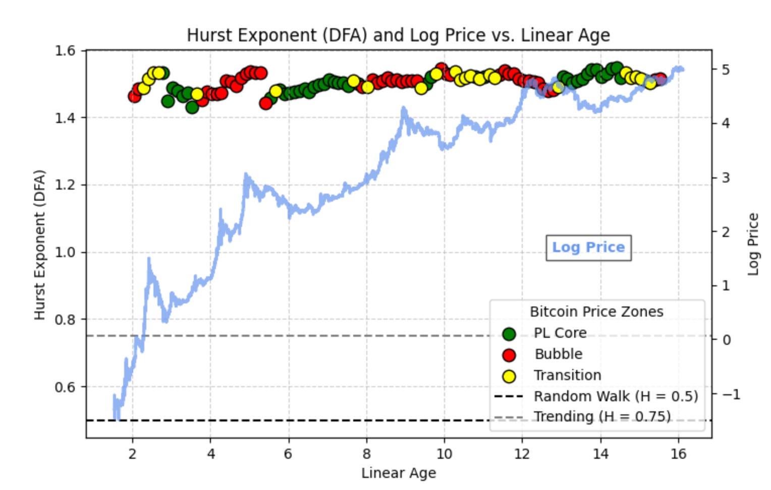
One sees some differences between the DFA linear and DFA quadratic method charts in Figures 4 and 5, but the results are broadly similar. The Hurst exponents are very high, always above 1.3 and generally above 1.4. Interestingly they do not fall with time, in fact appear to rise somewhat in the quadratic case. For the linear case, whose chart seems a little bit better behave, a next bubble price peak extrapolated date is around August 21, 2025.

Such high values indicate very strong trend-following or explosive behavior, what has been termed a super-diffusive process.

As a further check I performed the same DFA on 10 years of recent daily stock price data, using the SPY ETF. Stock prices tend to grow exponentially over long time periods, reflecting both monetary debasement and real growth, and for the data set examined the compound annual growth rate over the 10-year period was 11.4%. The fit to an exponential relationship gave R² of 0.93 for the SPY history. The log price residuals were calculated by removing the long term exponential relation (not a power law sine stocks do not behave in that matter). The DFA analysis of the residuals found H = 0.17 for the linear technique and 0.19 for the quadratic technique. These values indicate very strong mean reversion, in sharp contrast to what we see for Bitcoin.

Both the R/S and DFA techniques indicate very strong persistence, continued high alpha if you will, for Bitcoin. We lean more toward the R/S values as more conservative in this case, but it is good to have confirmation of the strong trending nature from the DFA analyses also.

Multi-fractal DFA

Next I examined Bitcoin to determine whether it is multifractal, with different behavior relative to small and large fluctuations. One determines a Generalized Hurst exponent and it is plotted against the multi fractal order q.

The parameter q controls how different sized fluctuations are weighted, q > 0 gives more weight to large fluctuations, q < 0 to small ones. The method follows the same procedure as described above for DFA but calculates many versions of the F fluctuation function not as the regular r.m.s. but as the r.m.s to the 1/q power (for the special case of q = 0, a log averaging is used).

Then one has a power law relation F(q,s) ~ s^H(q) . And if H(q) varies with q one has a multifractal series.

Figure 6. The generalized Hurst exponent as a function of multifractal order q. We have analyzed for each of the 3 zones. The bubble zone has somewhat higher values, especially for q > 0 corresponding to large fluctuations. The transition zone behaves more like the power law core zone except for very small q, the smallest fluctuations.

Figure 6 shows the results, divided by power law core, transition, and bubble zones in the usual manner. The series are highly multifractal with a range of about 0.4 to 0.5 variation from the smallest q (smallest fluctuation scale) to the largest q.

For the q < 0 small fluctuations, whether power law core, transition, or bubble zone, the trend persistence is high. For q ~ 1 to 2, one has H close to 0.5 or random walk behavior and for larger q, representing the largest fluctuations, the behavior is quite mean reverting, with H = 0.4 or less.

The power law and transition zones are more strongly mean reverting for large fluctuations. Trend following at small scales builds up smaller and then a “wave is caught” and larger bubbles can grow rapidly, and within the bubble zone fluctuations appear to collapse more slowly than they rise. Moderate-scale fluctuations can spend a lot of time close to random walk behavior, but large fluctuations can mean revert (back to the power law core) strongly.

Summary

While earlier studies using moving average and other detrending methods to estimate the Hurst exponent have found Bitcoin possesses H ~ 0.6 typically, we find much higher values of H when detrending using the long term power law behavior (by subtracting out the power law quantitative regression median trend from the log price series). I find H ~ 0.9 using the R/S technique and around H ~ 1.4 using the DFA method of estimating the Hurst exponent.

With sliding windows of one-year width the H values remain high and similar across the full time 15-year interval studied. Peaks in H appear to lead large bubble price peaks by over one year.

Bitcoin also displays substantial multi fractal behavior and we have examined that for each of three regimes: the core power law foundation, the transition regime, and the bubble zone. The generalized Hurst exponent has similar behavior as a function of multifractal order for each, with a somewhat larger gradient for the first two zones. Trending is high for small scale fluctuations and for the largest fluctuations mean reversion is clearly in force.