Log-Log-Log Candlesticks: Scale-Invariant Bitcoin Charts

Triple Log Candles and Growth-Optimal Kelly Criteria

Executive Summary

Bitcoin has been shown in numerous studies to approximately follow a power-law relationship between price and network age. In this article we employ a third logarithmic transformation by constructing candlesticks that occupy equal intervals of logarithmic time. These Log-Log-Log Candles represent equal multiplicative expansions of Bitcoin’s lifetime rather than equal calendar intervals, producing a scale-invariant representation of market history.

The resulting candles reveal a remarkably consistent geometric structure across Bitcoin’s evolution. Bull and bear markets become directly comparable despite spanning vastly different calendar durations. Ordinary least squares, quantile regression, and two candle-based regression methods all recover nearly identical long-term trends, demonstrating the robustness of Bitcoin’s power-law growth.

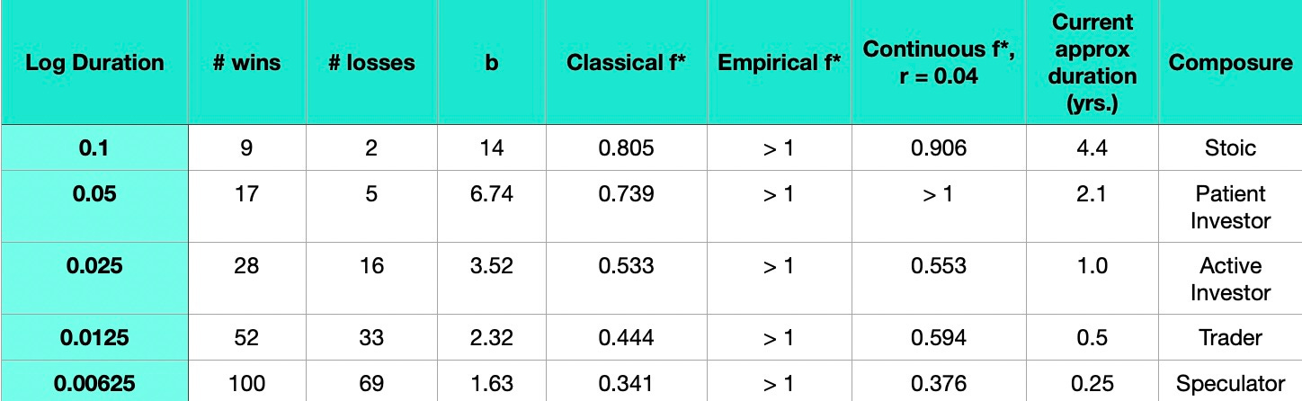
The candle construction also provides a natural framework for estimating growth-optimal portfolio allocation. Classical Kelly, empirical Kelly optimization, and continuous-time Kelly estimates were computed across multiple candle resolutions. The optimal classical Kelly fraction declines from approximately 0.81 to 0.44 as candle width decreases, and the continuous estimates are roughly consistent with the classical method. The empirical optimization remains at the 100% allocation constraint throughout the historical sample. Together these results indicate that Bitcoin has historically supported an unusually large growth-optimal allocation compared with conventional financial assets and that the finer log-time candles approach a stable continuous-time limit.

Log-log-log Candles

I introduced triple log candle charts for Bitcoin in a Substack article five months ago. Such a presentation is especially appropriate for long-term power law behavior. The two axes of price and Bitcoin age are logarithmic, but the duration of each candle is also logarithmic in time with the later candles much longer in duration than the earliest ones.

Each candle in the graphs below aggregates all daily prices that fall within a fixed interval of log10(age). As Bitcoin ages, each candle spans a longer period of calendar time, but the same fractional increase in age; this is a deliberate choice given the power law nature of Bitcoin. The plots are log10 in price on the y-axis and log10 in age on the x-axis; the current age of 17.5 years corresponds to a 1.24 log10 value.

The advantage of this triple log candle method:

* Calendar candles compress early history into only a handful of observations.

* Log-time candles distribute observations much more uniformly.

* Bubble and bear markets from different eras exhibit striking geometric similarity.

* Market structure becomes independent of Bitcoin’s age.

This chart style asks “What happened during one multiplicative stage of Bitcoin’s life?”

Below I present charts with increasing resolution starting from 0.1 in log10 of age, then 0.05, then 0.025, and finally 0.0125 in log10 terms. The final candle in these four cases is around 4 years long for the first chart, then 2 years, 1 year or 1/2 year in length respectively for the subsequent charts.

Figure 1. Log-Log-Log Bitcoin Candlesticks (Δlog₁₀(Age) = 0.10). Bitcoin price is plotted in logarithmic price versus logarithmic network age, with candlesticks constructed from equal intervals of log₁₀(age), corresponding to approximately 4.4-year investment horizons at the current epoch. Unlike conventional calendar candlesticks, each candle spans an equal multiplicative increase in Bitcoin’s age, producing a scale-invariant representation of market history. Green and red candles denote positive and negative net returns over each log-time interval, while the wicks indicate the full price range within each candle. The ordinary least squares (black dashed) and median quantile regression (purple dash-dot) from prior power-law fits closely coincide across the full history, demonstrating the robustness of Bitcoin’s long-term scaling behavior. The predominance of green candles (9 versus 2 red) reflects Bitcoin’s persistent secular appreciation over these logarithmically equal investment horizons and motivates the high growth-optimal Kelly allocations reported in Table 1.

Figure 2. Log-Log-Log Bitcoin Candlesticks (Δlog₁₀(Age) = 0.05). Bitcoin price is plotted in logarithmic price versus logarithmic network age, with candlesticks constructed from equal intervals of log₁₀(age), corresponding to approximately 2.1-year investment horizons at the current epoch. Unlike conventional calendar candlesticks, each candle spans an equal multiplicative increase in Bitcoin’s age, producing a scale-invariant representation of market history. Green and red candles denote positive and negative net returns over each log-time interval, while the wicks indicate the full price range within each candle. The ordinary least squares (black dashed) and median quantile regression (purple dash-dot) from prior power-law fits closely coincide across the full history, demonstrating the robustness of Bitcoin’s long-term scaling behavior. The predominance of green candles (17 versus 5 red) reflects Bitcoin’s persistent secular appreciation over these logarithmically equal investment horizons and motivates the high growth-optimal Kelly allocations reported in Table 1.

Figure 3. Log-Log-Log Bitcoin Candlesticks (Δlog₁₀(Age) = 0.025). Bitcoin price is plotted in logarithmic price versus logarithmic network age, with candlesticks constructed from equal intervals of log₁₀(age), corresponding to approximately 1.0-year investment horizons at the current epoch. Unlike conventional calendar candlesticks, each candle spans an equal multiplicative increase in Bitcoin’s age, producing a scale-invariant representation of market history. Green and red candles denote positive and negative net returns over each log-time interval, while the wicks indicate the full price range within each candle. The ordinary least squares (black dashed) and median quantile regression (purple dash-dot) from prior power-law fits closely coincide across the full history, demonstrating the robustness of Bitcoin’s long-term scaling behavior. The predominance of green candles (28 versus 16 red) reflects Bitcoin’s persistent secular appreciation over these logarithmically equal investment horizons and motivates the high growth-optimal Kelly allocations reported in Table 1.

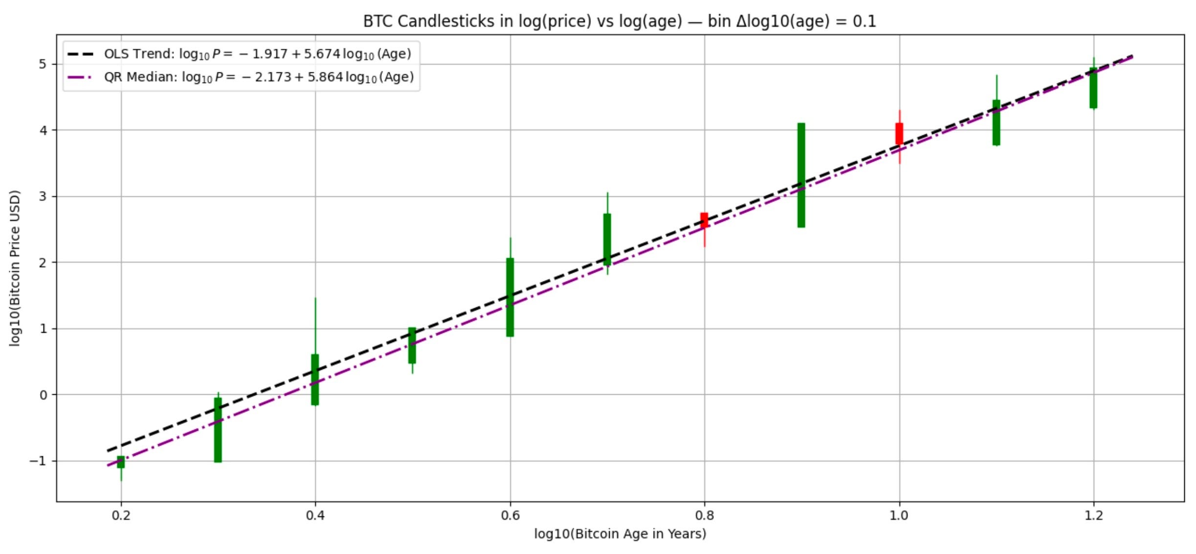
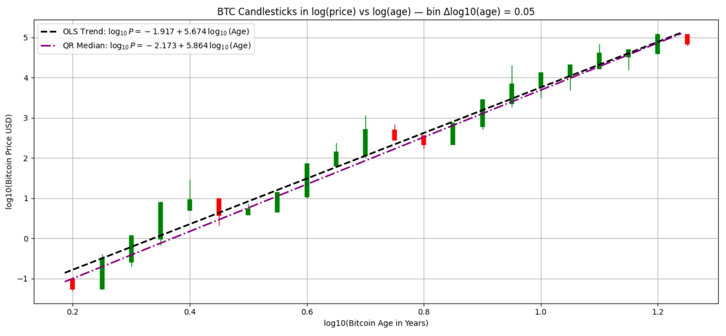
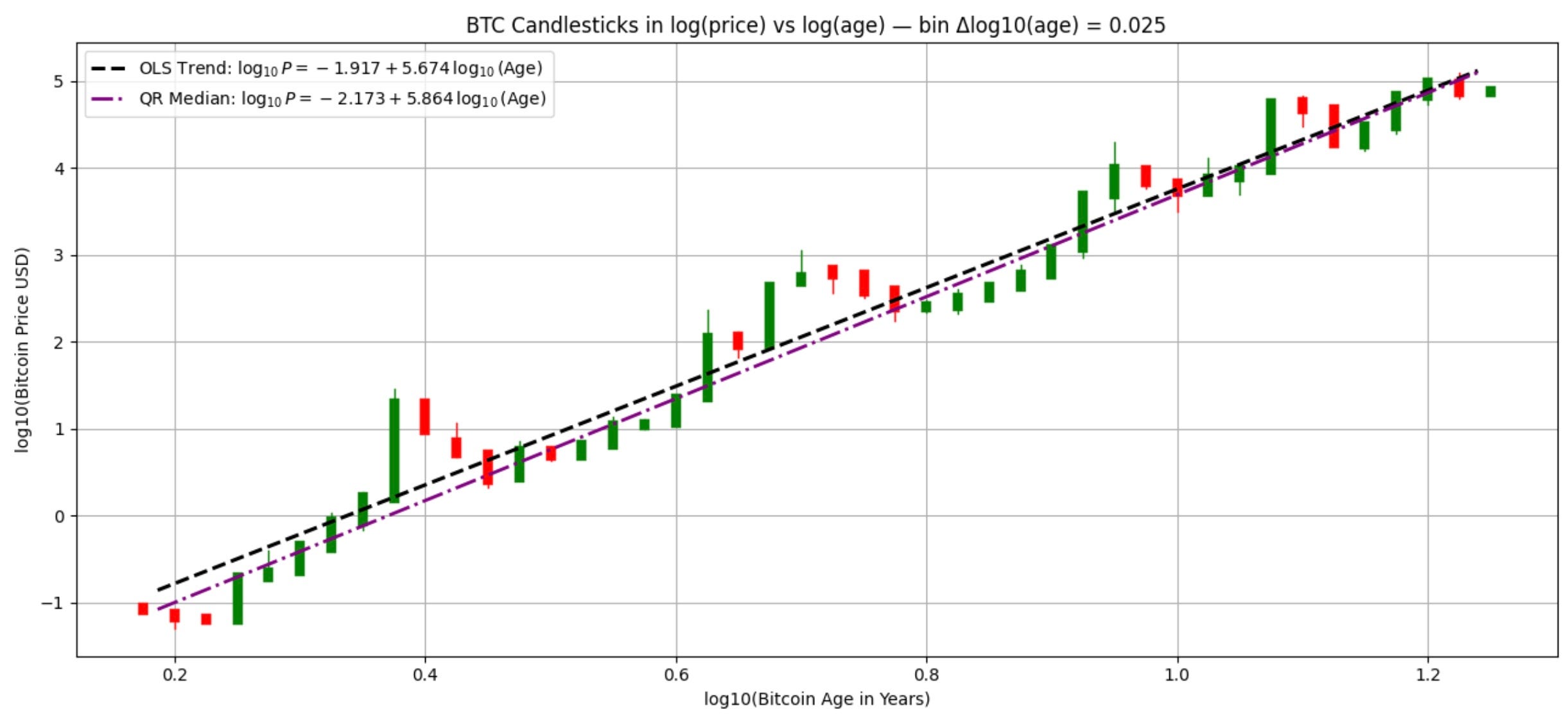
For the first three charts I also display previously determined OLS and QR regressions of log price vs. log time appearing as straight lines on these log-log plots, with similar slopes of 5.67 and 5.86 respectively corresponding to their respective power law exponents. One notices that the ratio of green to red candles is highest for larger values of the candle duration and bubbles become more apparent with shorter duration candles.

For this next highest resolution shown fourth chart, instead I have plotted two candle-based regressions: (1) using the geometric mean value (log midpoint) for each candle, and (2) determining a best fit through the candles using sum of least squares weighting for candles outside the best regression line. These produce very similar results, on top of each other in the graph with slopes of 5.84 and 5.88 respectively.

Figure 4. Log-Log-Log Bitcoin Candlesticks (Δlog₁₀(Age) = 0.0125). Bitcoin price is plotted in logarithmic price versus logarithmic network age, with candlesticks constructed from equal intervals of log₁₀(age), corresponding to approximately 0.5-year investment horizons at the current epoch. Unlike conventional calendar candlesticks, each candle spans an equal multiplicative increase in Bitcoin’s age, producing a scale-invariant representation of market history. Green and red candles denote positive and negative net returns over each log-time interval, while the wicks indicate the full price range within each candle. Unlike, the prior three plots using prior regressions, two regressions were performed on the candles themselves. One used the geometric mean midpoint for each candle and the second regression directly optimized the line passing through the candlestick bodies by minimizing weighted least-squares distances between each candle and the fitted trend. The two methods land on top of each other with slopes of 5.84(5.88) and R² values of 0.97 (0.98). The predominance of green candles (52 versus 33 red) reflects Bitcoin’s persistent secular appreciation over these logarithmically equal investment horizons and motivates the high growth-optimal Kelly allocations reported in Table 1.

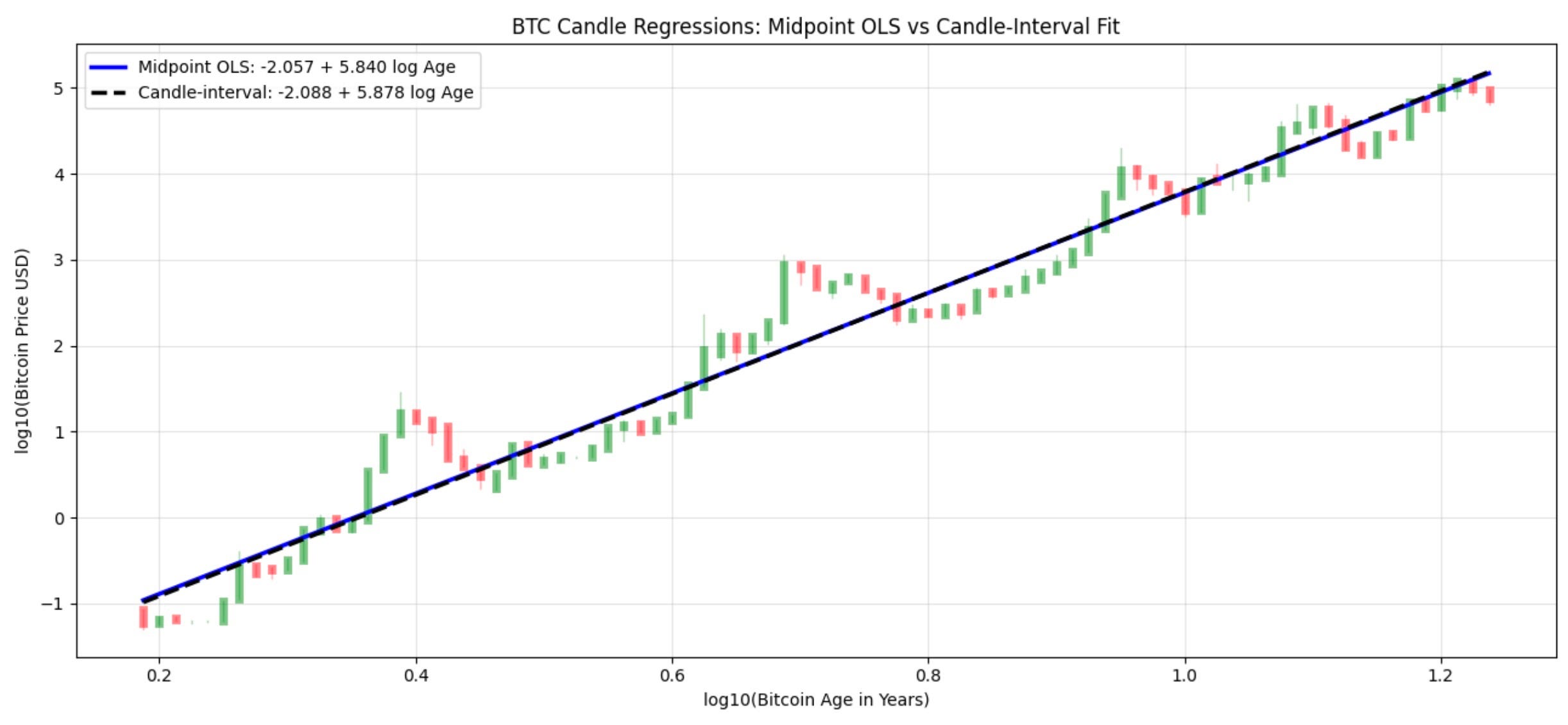
Indeed, all four regression methods (OLS, quantile regression, and these two candle regression methods) recover essentially the same long-run power law, indicating that the observed scaling is not an artifact of the regression technique.

Kelly Criteria (three methods) vs. Log Time Window

Log-time candle width naturally defines an investor’s time horizon. As the candles become progressively finer, the corresponding investor archetype transitions from the Stoic investor, who views Bitcoin over multi-year adoption cycles, to the Speculator, who experiences predominantly short-term volatility.

I employ three Kelly methods, each has a different philosophy:

• Classical Kelly is deliberately conservative

• Empirical Kelly simply asks: “What allocation would have maximized realized geometric growth?”

• Continuous Kelly incorporates the first two moments of returns

Despite their differences, all indicate historically high optimal allocations relative to traditional asset classes.

The three approaches answer slightly different questions. Classical Kelly depends only on win probability and payoff ratio. Empirical Kelly directly maximizes realized geometric growth over the historical return sequence. Continuous Kelly approximates optimal allocation using only the first two moments of returns.

The results displayed are the full Kelly allocations and investors often look at fractional Kelly, e.g. half-Kelly would be determined by multiplying the entries in the table below by 0.5.

Comparing the classical and continuous results we see 0.8 to 0.9 (80% to 90%) full Kelly allocations for the longest duration candles falling to 0.36 on average for the shortest candle study. One should realize that approaching the full Kelly is a little like approaching the summit of a hill, that while optimal, can see returns that fall sharply as one exceeds those full Kelly allocation values. It is interesting however that even the shorter one year durations at present suggest allocating up to half of one’s capital to Bitcoin relative to cash or T-bills.

All of the Kelly methods if put into practice assume regular reallocation to the new f* , which is to be updated as each candle closes. Here I have included partial (unclosed) candle results using the final candles of each series.

Table of Kelly results

Table 1. Three full Kelly optimal log growth f* methods, for each of 5 log-log-log candle series. The longer the log duration, the higher the f* allocation regardless of method. The classical method is p - q/b where p is the percentage of green candles, q the percentage of red candles, and b is the average win size vs. the average loss size. The empirical formula uses the observed return series: expected value of the sum of ln (1 + f R) where f is the allocation and R is the set of returns. The optimization for the empirical f* was bounded to not allow leverage, a maximum 100% allocation; all runs hit the upper bound. Continuous f* is calculated using the mean return (less a risk free rate r = 4%) divided by the variance.

Conclusions

The principal contribution of this work is the introduction of scale-invariant candlesticks. Once market history is represented in equal intervals of logarithmic age, Bitcoin’s geometric self-similarity becomes immediately apparent. The Kelly analysis follows naturally from this representation by treating each log-time candle as a standardized investment horizon.

The overarching contribution is not simply a different chart type. Triple log candlesticks provide a natural multiscale framework for analyzing Bitcoin. They preserve the network’s intrinsic scale invariance, produce robust estimates of the long-term power-law trend, and define investment horizons that map directly to growth-optimal portfolio allocation.

As candle widths become finer, the continuous Kelly estimates converge while the empirical optimization consistently favors full investment over the historical sample. Classical Kelly estimates are higher for investors with longer term outlooks. Taken together, these results suggest that Bitcoin’s long-run dynamics are unusually well suited to scale-invariant analysis and support substantially higher growth-optimal allocations than are typically observed for conventional financial assets.

This article presents historical statistical analysis rather than investment advice. Stephen Perrenod is engaged in econophysics research as a founder and Associate Director at the Scientific Bitcoin Institute.