Bitcoin’s Wealth Distribution

Not really a power law of wealth, yet

Wallets vs. Size

Bitcoin has been criticized for its top heavy wealth distribution. It is without a doubt top heavy, but less so after correcting for custodial holdings. The main categories for those are: (1) exchanges, (2) ETFs, (3) corporate holdings, and (4) government holdings, including government pensions. Other categories include sovereign wealth funds, hedge funds, and bank custody.

In this article I look at the known raw distribution and then approximately correct for the largest custodial positions. It is not a straightforward process, so the method is admittedly crude, but it illustrates the point of better balance than is seen in the unevaluated data.

There are two points that I wish to make in this article. One is that the wallet distribution has been getting gradually broader with time as shown in Figures 1 and 2. The second is that the distribution of beneficial ownership is different from the wallet distribution, after correcting for the largest custodial holdings. And the division between the richest wallets and others is lower when custody and beneficial ownership are taken into account.

Figure 1. A graph of the number of Bitcoin wallets above each of 7 thresholds as a function of time. The thresholds start at 0.01 BTC and each threshold is a factor of 10 higher. One readily sees that most of the relative growth for the past decade has been in the smaller balance wallets.

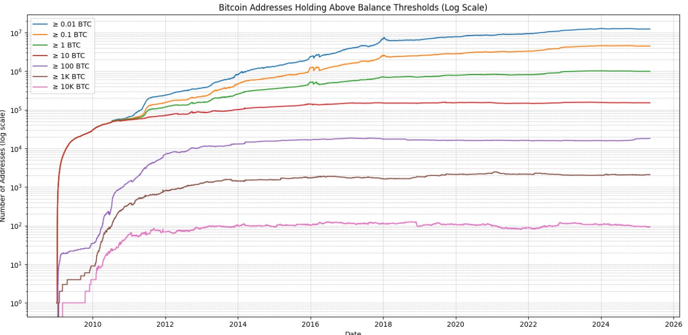
Figure 1 is a log-linear plot of the Bitcoin wallet balances over time. This has no correction for custodial ownership. These are cumulative balances above thresholds of 0.01 BTC or more, at each decade level up to the highest 10,000 BTC and above level. One sees that the fastest relative rise in recent years has been in the three lines representing balances below 10 BTC.

In Figure 2 we have plotted the best fit power law index for the number of addresses vs. minimum wallet balances, shown as a function of time. It is an inverse power law; the y-axis shows the absolute magnitude of the power law index. It ran up to 0.8 very early, fell back to the 0.6 neighborhood and has been rising since 2011 to over 0.8. Thus the distribution has been getting broader over time, with relatively more holdings at lower balances as is also seen in Figure 1.

Also plotted is the R² value, correlation squared or a measure of the goodness of fit. It has risen from 0.8 to a very respectable value in the high 0.9x range.

Figure 2. Best fit power law index to the cumulative address distribution as a function of time. After shooting up to 0.8 and then falling back below 0.6 around 2011, it has been on a steady climb to a more balanced distribution, rising above 0.8 five years ago.

Pareto alpha and GINI coefficients

Wealth and income distributions are often modeled by what are known as Pareto alpha (α) and GINI coefficients. In order to determine the Pareto α, we should plot the cumulative Bitcoin held above each bin level. In order to match the total supply of 19.86 billion Bitcoin we use a normalization factor of 2.78 to represent the midpoint of each bin, that is the 1-10 BTC bin has an effective midpoint of 2.78 BTC as the average holding for that bin, and similarly for the other bins.

Figure 3. Lorenz curve for the Bitcoin distribution reported at bitinfocharts.com.

The GINI coefficient for wealth distribution is only well defined for Pareto α > 1, and as we shall see our α values are much below one. Effectively the GINI is maximal at 1, highly unbalanced, with the Pareto approximation in such a case.

However one can calculate GINI more directly from the percentage of Bitcoin per bin and the percentage of addresses per bin. If you do that for the full Bitcoin distribution shown at bitinfocharts.com you find a GINI coefficient of 0.99. The GINI value calculates how full the shaded green area in figure 3 is relative to the entire lower triangle, which in this case it almost completely occupies. Bitcoin has a Lorenz curve that is very far removed from the diagonal ‘equality’ line.

Wealth distribution charts

Now let’s look more closely at the actual wealth distribution, basically the number of wallets for a given bin times the average balance per wallet in that bin and then accumulated appropriately for the threshold. As mentioned, we approximate the average balance in a bin by 2.78 times the lower bound, from our normalization procedure. This is close to the geometric mean of the bin lower and upper boundaries.

Figure 4. This chart shows on a log-log basis the cumulative wealth (orange line) vs. the average balance for each bin. Also shown is the best fit power law (red dashed line), which has a power law slope of -0.128. The Pareto α (alpha) is the absolute magnitude, 0.128. The 50% wealth level is in the vicinity of 1000 Bitcoin held. Source of data is bitinfocharts.com

Figure 4 plots the distribution, shown as an orange line for the log wealth per bin (measured in Bitcoin) vs. the log of the average holding in that bin. The red dashed line is the best fit power law of index -0.13 and thus by definition Pareto α = 0.13. This corresponds to a GINI coefficient > 1, very unbalanced. It’s not a great fit, with R² of 0.74, clearly the actual distribution tapers off at both ends. It must do so at the high end given the finite available number of Bitcoin, 19.86 million at present.

The 50% wealth level is at about 1000 BTC; that is half of all the Bitcoin wealth is held in wallets of that size or larger. This can be seen by looking at the log = 7 level on the y-axis that corresponds to 10 million Bitcoin, half are above that line, half below and the orange curve at a level of 7 is intersected by the line for 3 on the x-axis corresponding to 10³ = 1000 BTC.

Custodial allocations

In order to correct for custodial holdings we looked at all wallets greater than 40,000 BTC, most of these can be mapped to exchanges. We subtracted all of the identified large holdings from the >10,000 BTC bucket and reallocated the balances to their client populations. This process included also the known holdings of the largest ETFs (4), companies (Microstrategy and MARA), and governments (US, UK, China) with balances above 40,000, and those were subtracted from the highest balance bucket of total coins held.

We then evaluated the number of customers or share holders for all of these large exchanges, ETFs, and the two largest Bitcoin treasury companies, MicroStrategy and the miner MARA. Not knowing how to distribute their balances we placed the number of clients and their average balance entirely in the relevant bin based on average holdings per client.

We also did this for the three governments with balances above the 40,000 threshold. For these we took the population of each nation and distributed the holdings equally for the population, e.g. about $57 in BTC value per American. When we added up all the Bitcoin balances they were higher than 19.86 million, the current total.

Figure 5. The curve of cumulative Bitcoin relative to the midpoint for each bin (orange) and the best fit power law with Pareto α of 0.114, little changed from Figure 4. The R² is slightly poorer than in Figure 4. However the 50% level balance is decreased to around 300 BTC.

So I applied a renormalization process to the distribution, on the basis that the number of exchange customers and ETF customers is quite possibly overestimated. We scaled those back in order to match the current total bitcoin supply of 19.86 billion.

The result of this redistribution to client beneficiaries is shown in Figure 5. The adjusted cumulative wealth curve is in orange. The red dashed line is the best fit power law, with index -0.114 or Pareto α of 0.114. This is still very unbalanced, and little changed from before. Again a power law is not a very good fit.

The GINI coefficient calculated from the data (not from the α estimator) turns out to be 0.96, only slightly lower than before.

However, the 50% wealth level decreases considerably in this case, down to around 300 BTC. If the US were to fully fund its Strategic Bitcoin Reserve at 1 million BTC, up from the current initial 0.2 million, the 50% of all wealth point would be lowered further to around 250 Bitcoin.

The overall situation is that Bitcoin is quite closely held, but gradually becoming more broadly held. The existence of ETFs and stocks like MicroStrategy, and the moves toward holdings by pension funds and governments is also broadening passive ownership as a well as providing new channels for active participation in Bitcoin.

Only 1% roughly of the population ‘gets’ Bitcoin. Now gradually more and more are passively having some stake in the emerging Bitcoin economic system through governments and holdings of Bitcoin treasury companies in mutual funds.

If people come to understand the power law nature of Bitcoin price (only a few percent at best of Bitcoin holders ‘get’ the power law) perhaps more of them will move more of their savings toward Bitcoin, since the power law indicates 41% annual trend growth for now, and above 20% annual expected price increases between now and 2040.