Bitcoin’s Velocity Power Law

Derived not from Price but from Velocity

Figure 1. Quantile (QR) and ordinary least squares (OLS) regressions of Bitcoin price in a log-log chart, and thus the straight lines represent power laws. The OLS black line slope is 5.69, while the QR slope for the median 0.5 level (red solid line) is 5.83.Ordinary Least Squares and Quantile Regression of Power Laws

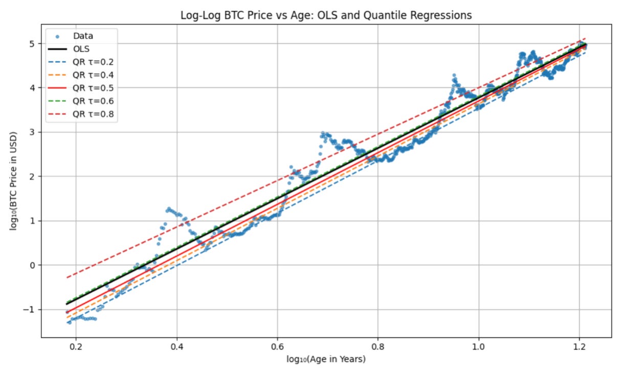
Ordinary Least Squares and Quantile Regression

Typically we derive the power law relationship for Bitcoin by simply looking at the price vs. age; this follows usual power law math with a normalization constant C and a power law index k (slope on a log-log plot) of

P = C * T^k,

where P is price and T is the Bitcoin network’s age, now over 16 and 1/2 years.

And regressions are generally performed as either OLS, ordinary least squares, or QR, quantile regressions. The OLS provide the mean value vs. age and QR at the 0.5 level provides the median.

Table 1. ChatGPT comparison of ordinary least square (OLS), quantile regression (QR for median), and Velocity methods of measuring the Bitcoin power law index k.

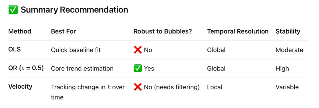
In the chart above the OLS regression yields a slope of k = 5.69 and the QR a slope of k = 5.83, and with somewhat different values for the constant C. The two techniques have relative tradeoffs, according to ChatGPT the QR method is more robust to bubbles and has higher stability. Both provide a global view.

Velocity Technique

There is a third technique, which uses Bitcoin’s price velocity rather than prices. How much does price change in a given time span? This technique can be performed by differentiating P = C * T^k and normalizing:

Differentiating yields dP = C * k* T^(k-1) and then dividing the left side by P and the right side by C * T^k results simply in

dP/P = k * dT/T.

That is, if one has a 1% change in the age of the Bitcoin network, the power law trend yields a k % change in the price. We can then calculate velocity dP/dT and compare to P and T at the start of an interval in order to estimate k.

The problem is that price is quite volatile, especially in bubbles, and velocities are even noisier. I have implemented two smoothing methods.

First method, 4 year averaging

Figure 2. The first velocity method. It uses 4-year windows centered around a date in question and then, because the intermediate result is quite noisy, a four year lagged average for smoothing.

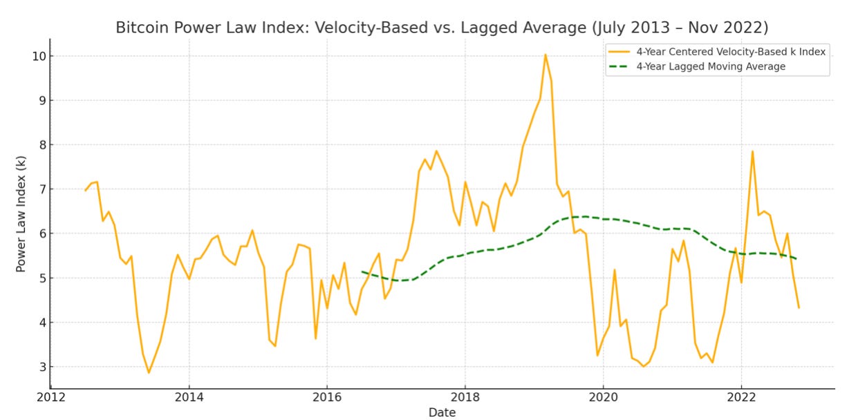
With this method, for a given date, I take a 4-year window centered on that date (2 years prior until 2 years after), and determine k from the Bitcoin change in price and age across the window. Four years was chosen since it is the typical interval between large bubbles. I then take that series, which is noisy, and average that with a four year lagging moving average. The result is the dashed green line. We see that it lies generally in the range from 5 to 6 for k and has settled to about 5.5, close to what is found from the straight OLS technique with prices.

Second method, all price history

Figure 3. The power law index as determined from the velocity calculation between the first price and age, and the price at some given time, as the endpoints. Despite filtering out much of the bubble behavior, there is still some evidence around 2011, 2013, 2017 of the bubble effects. But overall the index value (here called α) settles to around 6 for the past decade.

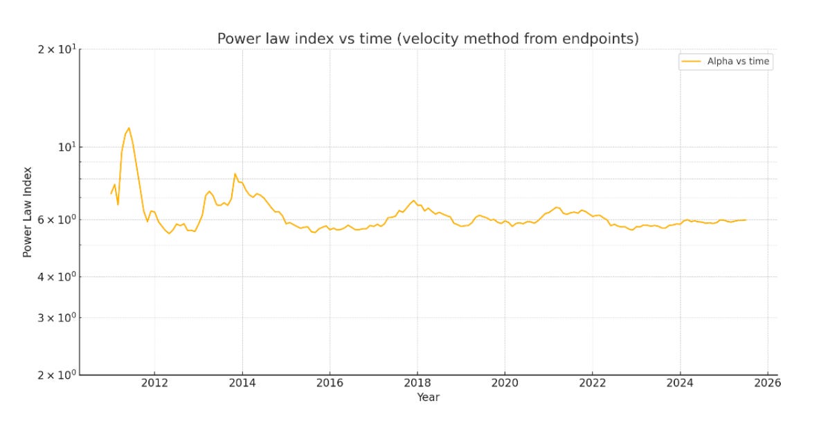
With this second method, I simply take the price ratio between the first data point and some particular date and take the ratio of Bitcoin ages between those as well. However, I first filtered out the bubble regions by running a QR first and using the points lying below the line. This would bias the result to somewhat higher values, but is needed for reasonable noise suppression. This results in the line in Figure 3.

While we still see some of the effects of bubbles in 2011, 2013, 2017, and to some extent in 2021, the overall power law settles down to close to 6 and has been more or less around that value for ten years.

Conclusions

All in all the agreement is good, with the first velocity method providing a power law index value slightly lower than the OLS technique, and the second method indicating a value somewhat higher than the QR technique.

The table above generated by ChatGPT notes that the velocity method is less stable, nevertheless we are able to obtain consistent results with all three techniques.

All of the techniques are consistent with the power law theory for Bitcoin as propounded by Giovanni Santostasi, based on Metcalfe’s Law, that applies to the Internet and to social networks and other networks that proliferate globally, allowing many-to-many interactions. Metcalfe’s Law says such a network’s value grows as close to the square of the adoption rate. Bitcoin’s adoption rate as measured by non-zero balance wallets has been measured by Giovanni and myself to be around the cube of the age of Bitcoin.

The Power Law Theory is thus approximately stated as:

Price ~ Adoption^2 ~ [(Age of Bitcoin)^3]^2 ~ Age^k, with k ~ 3*2 = 6. The square of a cube law goes as the sixth power.

And we can also support the power law theory by measuring k using the velocity of price vs. time as well as simply price vs. time regressions.