
Introduction
For years, Giovanni Santostasi — who first realized the power law nature of Bitcoin — and I have argued that Bitcoin follows this remarkably simple long-term relationship:
P(t) ~ tβ
where P is price, t is Bitcoin’s age, and β is the power law exponent, which is measured to be close to 6. A link to our scientific paper “A Mechanistic Derivation of the Bitcoin Price Power Law”, demonstrating the relationship via multiple methods, and posted at the CERN preprint site, is here: https://scientificbitcoininstitute.org/research/publications
Critics often respond with a reasonable objection:
Of course Bitcoin price rises with age. Both variables increase over time. But is the apparent relationship merely a statistical artifact? As time moves along all prices increase in dollar terms. Is Bitcoin just leveraged exponential growth?
This criticism deserves a serious answer.
To investigate, I analyzed the complete daily Bitcoin price history from Coin Metrics, spanning nearly sixteen years, from July 2010 through May 2026, comprising 5,789 daily observations.
The results were surprisingly strong.
The Power Law Fit
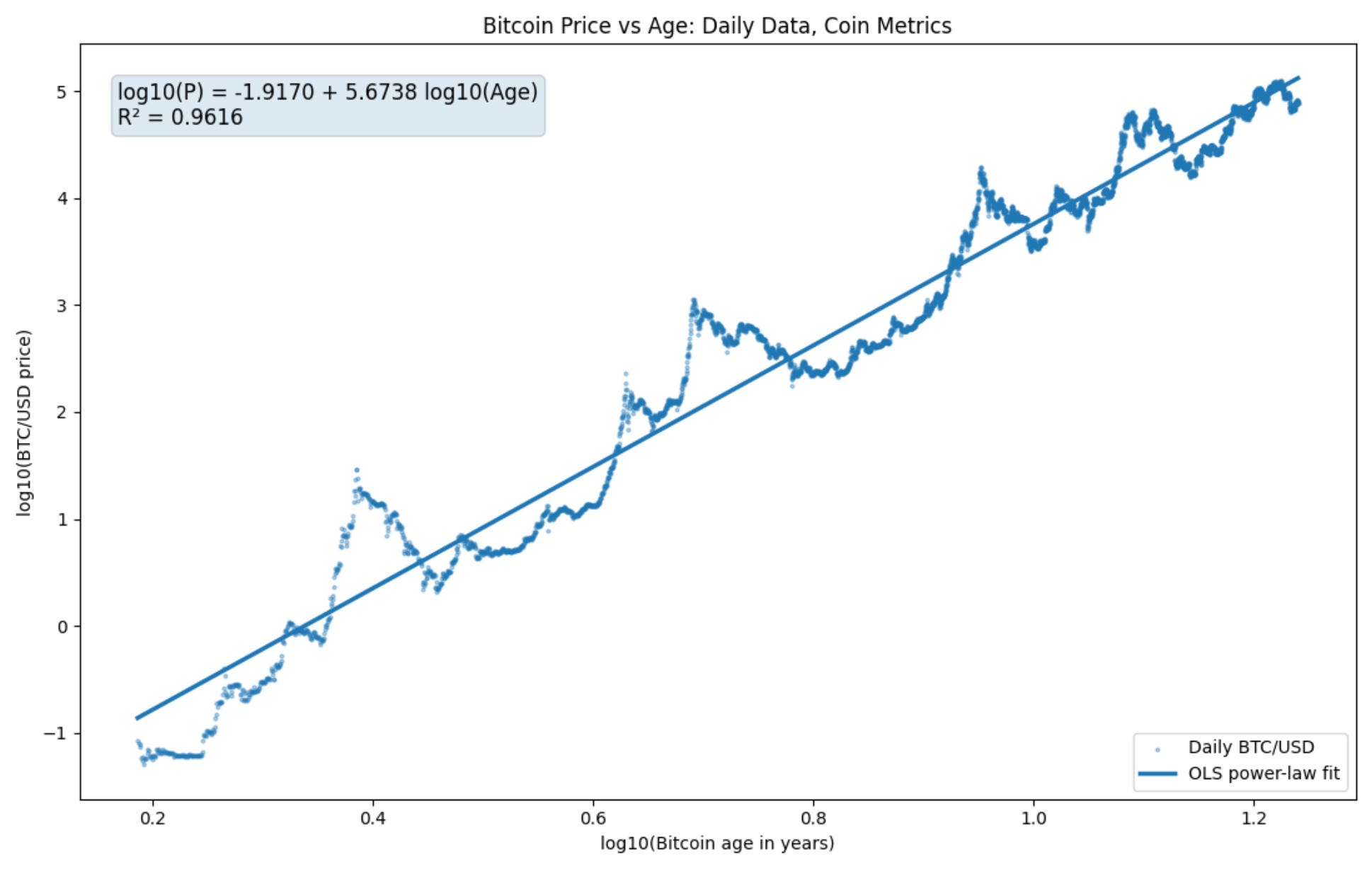
Using the entire daily history, the best-fit relationship for the dollar price is:
log (P) = -1.917 + 5.674 log (Age)
which corresponds to:
P = 0.0121 * Age^{5.674}
The model explains over 96% of the variation in Bitcoin’s logarithmic price history (all logs in this article are log base 10).
Attempts at an exponential fit for Bitcoin’s price history fail spectacularly, see Table 3 from the recent Baquero and Menezes paper https://arxiv.org/pdf/2605.21316 . Their fit of the power law with two parameters strongly outperforms an exponential fit with two parameters by an identical R2 = 0.96 vs. 0.87 for exponential, lower residuals of 0.30 in log price vs. 0.53, and most tellingly, by an enormous margin of 6480 points on the AIC (Akaike information criterion). Even a 100 point improvement is clear evidence of model superiority
Table 1. Power Law Fit (this article)
Quantity : Value
Observations : 5,789
Start Date : July 18, 2010
End Date : May 19, 2026
Power Law Exponent β : 5.674
R² : 0.962
An R² of 0.962 is impressive, but by itself it is not enough. Two variables can exhibit a high correlation while having no genuine long-term relationship. The key question is whether Bitcoin remains tied to the power law over time.
Dog Walking analogy
Imagine a dog walking beside its owner. The dog wanders left and right, sometimes far away, but remains attached by a leash.
Bitcoin’s price appears to behave similarly. The power law is the owner’s path, while the distance between price and the power law is the leash. During speculative bubbles the dog may sprint far ahead. During severe bear markets it may lag well behind. The owner is focused on the path forward.
The critical question is whether the leash actually exists. Does Bitcoin eventually return toward its long-term trajectory, or are the apparent power-law relationships merely a statistical illusion created by two quantities that both happen to increase through time?
Modern econometrics has tools specifically designed to test this idea.
The Statistical Tests
I used separate approaches on price and residuals.
Augmented Dickey-Fuller (ADF)
A test that asks whether a series tends to wander indefinitely or eventually returns toward a stable range.
Phillips-Perron (PP)
A more robust version of the same idea that better handles correlated noise and changing volatility.
Engle-Granger Cointegration Test
A test that determines whether two variables share a common long-term equilibrium even though both wander over time.
Step One: Is Bitcoin Price Itself Stable?
The answer is no. Both the Augmented Dickey-Fuller (ADF) test and the Phillips-Perron test indicate that Bitcoin’s logarithmic price is non-stationary.
A stationary series fluctuates around a relatively stable range. While it may move up and down, its statistical character remains broadly unchanged over time. A non-stationary series behaves differently. It can drift, trend, or evolve over long periods, so that its average level today may be very different from its average level years earlier.
Bitcoin clearly belongs in the second category.
Table 2. Bitcoin Price Tests
Test: Result
ADF on Log Price: Non-stationary
Phillips-Perron on Log Price: Non-stationary
First Difference of Log Price: Stationary
These tests indicate that Bitcoin’s price history is not simply oscillating around a fixed equilibrium value. Instead, the price exhibits a persistent long-term tendency to evolve over time.
Importantly, these tests do not tell us what form that evolution takes. They do not distinguish between exponential growth, power-law growth, random-walk behavior, technological adoption, or other possibilities. They simply tell us that Bitcoin’s price contains a powerful long-term trend.
The critical question is therefore not whether Bitcoin trends, but whether the particular power-law relationship observed between Bitcoin price and Bitcoin age is statistically meaningful.
If Bitcoin and age are merely two variables that happen to increase through time, the apparent power law could be a statistical illusion. To investigate that possibility, we remove the power-law trend and examine what remains.
Step Two: What Happens After Removing the Power Law?
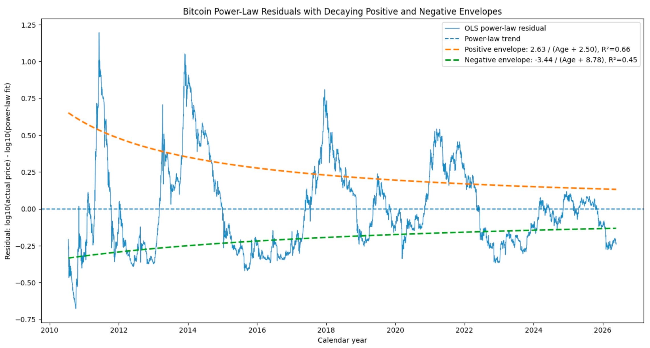
After fitting the power-law model and subtracting it from the data, I examined the remaining residuals—the deviations above and below the trend.
If the power law were spurious, these residuals would continue to wander indefinitely. In that case, the apparent relationship between Bitcoin price and age would have little statistical meaning.
Instead, the residuals become stationary.
Table 3. Residual Tests
Test : p-value, Result
ADF Residuals: 0.006, Stationary
Phillips-Perron Residuals: 0.024, Stationary
Engle-Granger: 0.026, Cointegrated
All three tests point in the same direction, and all three produce p-values below the conventional 5% significance threshold.
If Bitcoin’s apparent power law were merely the result of two unrelated quantities increasing through time, we would expect the deviations from the fitted trend to continue drifting without bound. Instead, the residuals pass multiple stationarity tests, while the Engle-Granger test finds a statistically significant long-term relationship between Bitcoin price and Bitcoin age.
In practical terms, Bitcoin does not appear to wander arbitrarily far from its power-law trajectory. Bubbles and bear markets occur, sometimes dramatically, but the departures remain bounded rather than exhibiting an ever-growing random drift. The evidence therefore supports the existence of a persistent long-term relationship between Bitcoin price and age rather than a spurious correlation between two unrelated trending variables.
The power-law trend acts as an attractor around which bubbles and bear markets occur.
This is the central result of the analysis. Bitcoin itself is non-stationary, but the deviations from a power-law function of age appear stationary. Multiple independent statistical tests support the conclusion that the observed power-law relationship is unlikely to be a spurious correlation between two unrelated variables that merely happen to trend upward over time.
A Note on Autocorrelation
The residuals are highly autocorrelated. In simple terms, today’s deviation from the power law is strongly related to yesterday’s deviation.
This should not be surprising. Consider a rocket following a trajectory to the Moon. If it is slightly above its planned path today, it will probably still be above that path tomorrow. Its position evolves continuously rather than resetting randomly each day.
Bitcoin behaves similarly. Adoption, capital flows, investor sentiment, and macroeconomic conditions evolve over months and years rather than changing instantaneously. As a result, deviations from the long-term power-law path exhibit persistence and memory.
Importantly, persistence is not the same thing as drift. A pendulum may have a highly predictable position from one moment to the next, yet remain confined within a limited range. In statistical language, such a process can be stationary even while exhibiting strong autocorrelation.
That appears to be the case for Bitcoin. The residuals are highly autocorrelated, but the stationarity and cointegration tests indicate that they remain bounded over the long run. Bitcoin may wander above or below its power-law trajectory for extended periods, but the deviations do not grow without limit.
Why This Matters
This does not prove that Bitcoin’s future price is predetermined. Nor does it prove that the power law must continue indefinitely.
What it does show is that the relationship observed over the last sixteen years is not easily dismissed as a coincidence produced by two variables that both happen to rise over time.
The power-law model survives multiple standard econometric tests designed specifically to identify spurious regressions. In particular, the Engle-Granger test rejects the hypothesis that Bitcoin price and Bitcoin age are unrelated long-term processes.
That result is important because it addresses one of the most common criticisms of power-law modeling.
What the Tests Do Not Say
These tests do not predict next month’s price. They do not identify cycle peaks. They do not explain every bubble and crash.
They simply address a foundational question: Is there evidence for a stable long-term relationship between Bitcoin price and Bitcoin age?
Based on sixteen years of daily data, the answer appears to be yes.
⸻
Stephen Perrenod researches the network economic and econophysics properties of Bitcoin, as Associate Director of the Scientific Bitcoin Institute.
Stephen, great presentation... clearly the power law is not broken.
Is there a formal statistical test that presents the latest date beyond which the latest historical stability cannot be correlated to current stability results? I recall a discussion on one of the yt channel episodes where you described the Lindy Effect and related it to that latest date ... something like: add 2 to 2-1/2 times the current age to the latest sample date. Beyond this calculated date, Lindy Effect cannot apply.
More to the point - while your conclusion that core PL cannot predict the tomorrow's price makes sense, the trend of past historical data shows statistical significance that, at any historical age, the range of data up until that selected range endpoint. For example, pick the a relatively early start date: 1 June 2013 as the start date and six years beyond for the range's end date: 31 May 2019. To what degree is core power law predictive to the historical samples of the following six years?
Your rocket to the moon analogy seems apropos. At non-relativistic speeds, the path of an undisturbed body "flying" between the earth and moon is highly predictable though with small errors in orbital parameters between t1 and t2. Spacecraft navigators take a celestial fix at t2, enter the fix info into their nav computer and the output is revised orbital parameters. Bodies orbiting our Sun describe an elliptical path that demonstrates PL behavior. The path of that planet/asteroid/dust particle around the sun is predictable enough with today's digital models. But 5 billion years ago, the path of objects orbiting the Sun must have been extremely unstable. Collisions abounded. Not nearly as unstable today. And the PL of semi-major axis distance vs orbital period for each planet displays a PL.
"Nobody can predict the future." But this claim, left alone, closes the eyes of the claimant to the reality of practical spaceflight today. Power laws that grow more stable over time seem to offer practical predictability.