Bitcoin Power Law with an AR(2)-corrected Generalized Least Squares Analysis
99.9% R-squared!? $300K possible in 2025
In October I wrote an article about generalized least squares regression of the Bitcoin power law. Normally what you see is OLS, ordinary least squares regression, which determines the mean trend, or quantile regression, which provides regression equations at a number of pre-defined percentile levels, such as 1%, 10%, 25 %, median, 75%, 90%, and 99%, or other selected values.
In many financial and economic time series there is auto-correlation; generalized least squares (GLS) seeks to correct for that. There are multiple techniques one can use, and in the October article I used an AR(1) correction, that corrects for auto-regression between a value at one time and the value just prior, e.g. the day before if daily values are used, a week prior if weekly values compose the data set.
In this analysis, and in October, I used the full available weekly price history for analysis. Here is a summary of what the AR(1) analysis in October found:
The AR(1) generalized least squares regression reduced the R^2 to 0.62, but the other statistical parameters were much improved. The Durbin-Watson (D-W) statistic increased to 1.75 from the 0.03 obtained with OLS, which value indicated high autocorrelation. A D-W value of 2 has no auto-correlation and a zero value indicates maximal positive autocorrelation. For the GLS regression the power law index steepened from 5.68 to 5.89 (with a standard error in slope of 0.17).
Now in the case of Bitcoin, autocorrelation is not a bad thing per se, nor does it invalidate the essential power law nature. Think of a rocket ship: it follows a trajectory for which the next location depends very much on the prior one, because of underlying physics. Bitcoin also has underlying physics since it is based on energy, cryptography, and Metcalfe’s quadratic (square of number of users) law for networks. The growth of Bitcoin adoption is itself near to a cubic power law. A quadratic of a cubic is a power law of index 6. Bitcoin’s power law is close to that level.
Nevertheless we would like to analyze the residuals and account for autocorrelation in order to better determine the underlying trend, and provide sensitivity testing to the overall power law relationship. Bitcoin also has exponential bubbles, during which autocorrelation tends to increase (some dare call this FOMO), and that applies on the way up and the way down back to the underlying long term power law behavior.
The GLS analysis is a multi-step procedure. One first runs an OLS regression and then examines the residuals for autocorrelation. The parameters of the autocorrelation are then fed to a generalized least squares regression (also called Feasible GLS = FGLS) analysis of the same price data set.
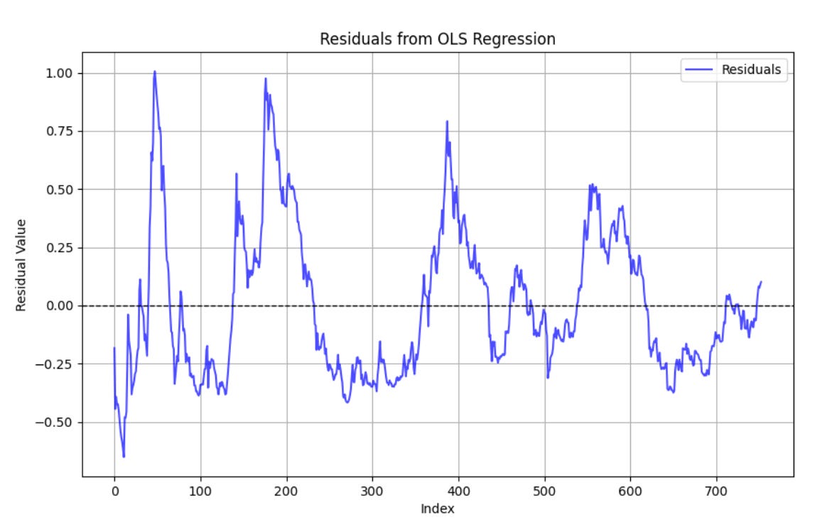
Figure 1 shows the log10 residuals of the OLS regression, where the x-axis is the age of Bitcoin in weeks. Currently one standard deviation is about 0.25 and two is about 0.5 in the log, and the residuals skew heavily to the right (positive) tail. Over the whole series, one standard deviation is about 0.31 in the log. Note the peaks in the residuals have decreased in height monotonically, volatility has been decreasing. Also you can see we are now only a little above fair value, even with Bitcoin’s recent price having breached $100,000.
The residuals were analyzed for AR(2) correlation including the prior price point from any given price value and the one prior to that as well, and the AR2 best fit equation is:
Residual(now) = 1.111 * Residual(last week) - 0.130 * Residual (two weeks ago) + 0.001

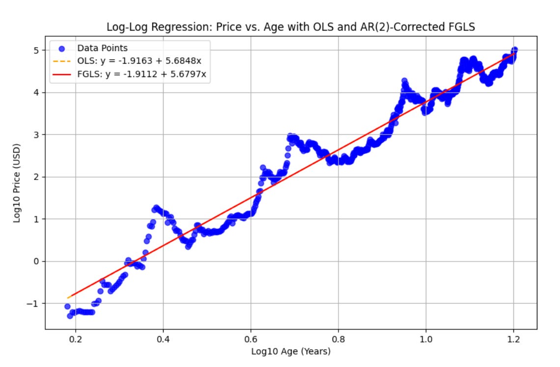
Figure 2 shows the best power law OLS fit and the FGLS fit on a log-log plot, including weekly data to the middle of December 2024. The power law slope is 5.68 as also found in the OLS analysis from October. The OLS is plotted as a straight dashed line and the FGLS regression using the AR2 fit to the residuals is plotted as a solid line. For this comparison, the power laws are basically right on top of each other. Both have slope 5.68 to within rounding, and very similar intercepts, thus only the solid line is visible except at the very earliest times. The standard error on the slope for the FGLS power law index is very small, at 0.01.

An exponential function does not fit this data in any useful way, it would be significantly curved on a log-log plot. The power law has persisted since around age three (log10 = 0.5 on the x-axis) for Bitcoin, after the first large bubble collapsed.
The FGLS regression has amazingly good statistics. R^2 = 0.999 (‘adjusted’ value is 0.999 also). The Durbin-Watson statistic is almost exactly 2, at 2.01 indicating autocorrelation fully corrected for. The log likelihood value is 1120 and the AIC -2237; both are improved from the October generalized least squares AR(1) analysis.
In order to test the very high R^2 value indicated, I also divided the data set into early years and late years in various ways and in all cases R^2 reached 0.99, the log likelihoods and AIC values were favorable, and the D-W statistic was close to 2.0. So why is R^2 so high for this model? According to ChatGPT 4o, that and the very high F-test value of 541,800 indicate that the independent variable (age) contributes significantly to explaining price behavior with these indications:
Strong log-log relation, Bitcoin follows a predictable power law relation
Narrow range for residual variance since AR(2) adjusts (ed. very well) for autocorrelation
If external factors align with age, the model can appear to explain all the variance
Log-log transform compresses variability

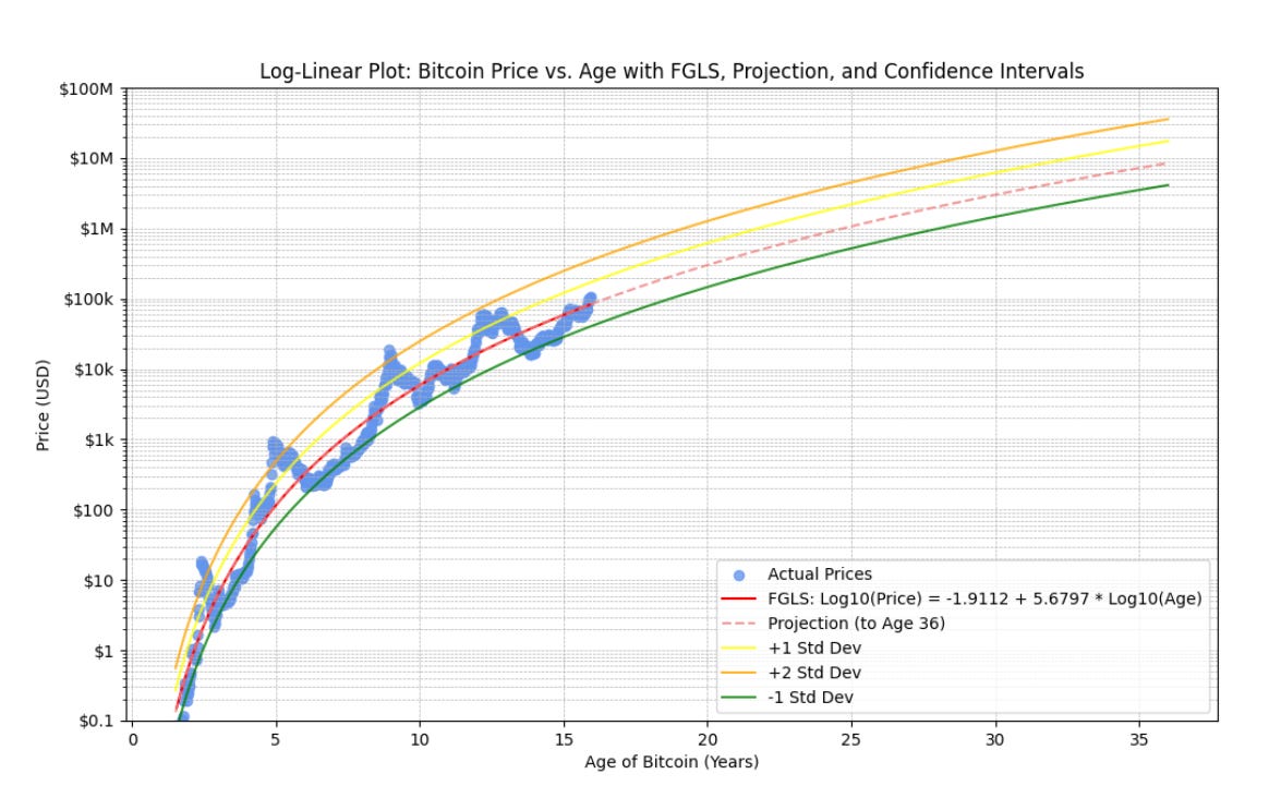
In Figure 3 we plot the same price data and the FGLS model projected to age 36 for Bitcoin (year 2045 start). We also show the +1, +2 standard deviation curves and the -1 standard deviation curve. And these are curves, not straight lines, because we are displaying power laws on a log price vs. linear time plot. (An exponential function of age would be a straight line on this plot).
The table below shows the expected year when the trend reaches some particular values, and also the earlier dates to reach such a price with a one sigma bubble or a two sigma bubble up in price, using 0.24 for log10 standard deviation of price. The choice of 0.24 is based on the (lower) volatility observed in the second half of the historical data. Of course the positive bubbles only occur every fourth year it seems, and if the pattern holds, the peaks would occur in years 2025, 2029, 2033, 2037, etc. There is no clear reason to think this will continue, the world is changing so very quickly and liquidity, election, and halving cycles differ in duration and phase.

Based on the projected dates in the table, the price level of $300K seems reachable in 2025, if there is a two sigma bubble, and if Bitcoin peaks mid-year or later in the year. Fair value with this model for January 2025 is $85K and for July, 2025 it is $101K, ignoring any exponential bubble up.
The downside (minus one sigma) for the trend values is a lower price by a factor of 10^0.24, which is 42% below the trend price associated with the date in the second column of the table, e.g. in the case of the second row with $1 million target price, then a price of around $580K if a bear market pulled back to minus one sigma for year 2033.7. So the full range possible for year 2033.7 is approximately [$580K, $3 million] since a two sigma bubble to $3 million could be reached by an earlier date during 2033, rather than 2039 as on trend.
Make volatility your friend. This article is not investment advice.

Outstanding work! A very insightful read.