Bitcoin Breaks $30K, Recovers

Don’t Over-invest Mentally in the Stock-to-Flow model

Breaking $30K is no big deal, long term

We broke $30K to the downside. This is not unexpected. Bitcoin’s price has rather quickly bounced back above that level, at least for now.

You may have followed the stock-to-flow model (S2F) and as a result have unrealistic expectations for nearly $100K or even $288K Bitcoin (S2FX variant model) this Halving cycle. But that model can never hold true in the long run. 

Here’s why: it has, in various versions, price or market cap as a power law with index > 3 and since the S2F is algorithmically slated to double every four years, it implies a power law of an exponential. And that is highly divergent mathematically. S2F heads toward infinity and a power law of a quantity approaching infinity grows much faster. The model fits historically, but the seeds of its destruction are baked in to the math.

In 2024 with the next Halving the stock-to-flow will hit 120, up from 57 today. A stock-to-flow of >100 corresponds to inflation <1%. That is uncharted territory for the S2F model, and once inflation has reached such a low value, Bitcoin’s low inflation in supply becomes far superior to fiat inflation. It is the differential with its competitor, fiat inflation (such as the over 5% recently recorded for the CPI index in the US) that is relevant in the long run for Bitcoin’s store of value capability.

For the intermediate term the spread of adoption, the network effect, is of great importance. Thus in this article I examine technological adoption-based models as well as supply-based models.

Bitcoin is for savings

Bitcoin is for the patient. HODLing is for the patient. Be stoic. Bitcoin is about low time preference, long time frames. It is long-term savings technology.

You must remember the volatility is high, over a factor of two standard deviation in any reasonable model, and that includes S2F. Get comfortable with that fact and use the convexity of Bitcoin to your benefit.

It is actually at $31,000 now, currently closer to fair value for several alternative models that are convergent or at least less wild than S2F.

It will likely grow substantially in the long term. This is a 500-year  breakthrough in monetary technology that is on roughly a 25-year or 30-year time scale before it reaches large scale deployment. 

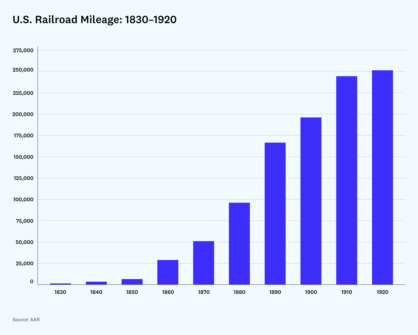
It took railroads in the US 60 years to level off in their expansion. To our benefit, technology moves faster these days.

 Block calendar and block years

All of the long term models discussed here use the Block calendar, with monthly intervals between data points starting from 2 Block years elapsed until the present 13.17 elapsed Block years.

Block years contain 52,500 blocks each and because average block times are usually somewhat less than 10 minutes, block years are slightly shorter than Gregorian calendar years.

So there is little difference these days between the length of a Block year and a calendar year. Average block time can and does depart somewhat from 10 minutes, but the difficulty adjustments regularly push the block time back toward 10 minutes on average. The difficulty adjustment is a key microeconomic process that drives adaptive behavior of the mining community between Halvings.

There are two classes of models discussed here, supply-based and technology adoption-based.

Supply-based models

The first class of models is based on the predetermined future supply. This is a great advantage compared to say commodities, whose future supply must be estimated. The future supply of Bitcoin is completely algorithmically determined, with the only uncertainty being average time for block creation and the difficulty adjustments smooth that out. Bitcoin has supply-demand economics like no other asset, with supply fully predetermined.

The S2F and Hybrid models explicitly include the Halving cycle through the S2F parameter. The Hybrid model has the same power law term as the S2F model but adds an additional term reflecting all future supply yet to be issued. So it combines both the differential and integral supply measures. It says that Bitcoin’s market cap depends on both supply rate (the differential) and the total of all future supply (the integral).

The best fit Hybrid model with 11 plus years’ of monthly data looks like this:

Log10 of Market Cap ($ billions) = 1.354 * Log10 of S2F - 4.424 * f + 0.7632

thus the relationship with S2F flattens to a more reasonable power law of index 1.35 rather than about 3.28 that is found for a pure price vs. S2F model. Both S2F and f, the fraction of the 21 million Bitcoin not yet mined, are functions only of the number of Block years elapsed. The second term incorporates the integral of all supply of unmined Bitcoin. It is an inverse exponential relationship with the market cap increasing as the unmined supply decreases. If there were no S2F term, the model would imply an asymptotic market cap value. The current fair value market cap from this model is $459 billion.

Technology adoption-based models

The second class of models is based on increasing technology adoption with time and implicity reflects network effects and supply changes as well. These other two models do not explicitly incorporate supply. The Lindy model is a power law model of price vs. time that is, conveniently, a good approximation to an S-curve in the domain t << characteristic time.

The S curve model requires a hypothesized asymptotic value and a shape parameter and a timescale parameter. Because we are in the early stages we cannot statistically discriminate by terminal value, but a model that goes to $30 trillion market cap has a 27 Block year characteristic time scale. We are not halfway there. A $100 trillion market cap model has a 33 year time scale until starting to level off. (The S-curve models use a Weibull cumulative distribution function in which the market cap reaches 63% of ultimate value at the respective time scale).

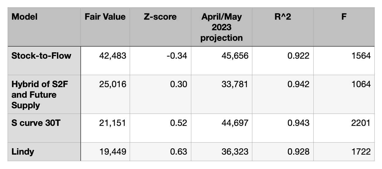
Table 1: Comparison of current fair value and 21-month predictions for four Bitcoin pricing models. The first two models are supply-oriented and the second two are technology adoption-oriented. The Z-score shows the number of standard deviations by which current price exceeds model price as of July 16, 2021. My regression for S2F yields a model fit fair value about half of that shown here: https://www.lookintobitcoin.com/charts/stock-to-flow-model/ . In part that is due to my use of forward looking S2F. S2F takes a quantum leap immediately at Halving boundaries. PlanB allows the model a one year ramp up with a 365-day backward looking average S2F. This seems like an artifice since S2F is completely anticipated by market participants. Also I use Block years rather than calendar years and monthly data rather than daily data since interested in the longer term fits. The Block calendar allows direct and precise calculation of the S2F parameter.

All four models have good values of R^2 correlation and very high values of the F-statistic and provide acceptable fits to the 135 data points with 2 or 3 free parameters. The p-values are all much smaller than 0.05 except for the intercept parameter in the Hybrid model which has p = 0.16. The S curve model has the highest value for each of R^2 and F.

Fair value for each of the three models that I have developed is currently in the $19K to $25k range, so we are not below fair value now. All models indicate that price is within a single standard deviation of fair value.

Don’t invest too much hope in models that forecast $100K or more this year. It could happen, given another bull run and volatility. But we would have to reach two or more standard deviations above fair value for more realistic models.

We are well within reasonable long-term model expectations. We may have seen the peak for this Halving cycle. It typically occurs 12 to 18 months after the halving and we are in month 14.  Accumulate and HODL for the long term, another Halving is slated for 2024. That will provide another shock-to-flow impulse, but it appears that each impulse is smaller than the prior one.